Today's topics are:
3D plotting
Matrix calculus
Borel summation of divergent hypergeometric series
Optional consistency with Mathematica
Internal reorganization
3D plotting
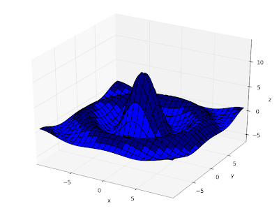
Jorn Baayen submitted a patch that adds 3D surface plotting (along with some other minor changes to the visualization module). Thanks a lot! I previously blogged about 3D plotting using matplotlib.
You can now easily produce plots of functions of the form z = f(x,y):
splot(lambda x, y: 10*sinc(hypot(x,y)), [-10,10], [-10,10])

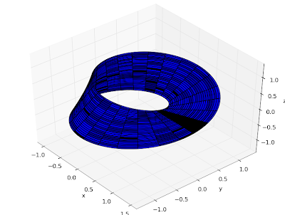
You can just as easily plot more general parametric functions x,y,z = f(u,v). The following plots a Möbius strip:
def f(u,v):
    d = (1+0.5*v*cos(0.5*u))
    x = d*cos(u)
    y = d*sin(u)
    z = 0.5*v*sin(0.5*u)
    return x,y,z

splot(f, [0,2*pi], [-1,1])

(I'm not sure why there are black spots in the image. This seems to be a matplotlib bug.)
Matrix calculus
It's now possible to compute exponentials, sines, cosines, square roots, logarithms, and complex powers (Az) of square matrices:
>>> mp.dps = 25; mp.pretty = True
>>> A = matrix([[2,3,1+j],[1,0,-1],[2,1,5]])
>>> nprint(expm(A))
[ (27.6034 + 41.2728j)   (24.9924 + 31.1189j)     (8.67256 + 68.271j)]
[(-15.0962 + 1.51713j)  (-10.1713 + 1.30035j)  (-28.7003 - 0.401789j)]
[ (125.368 + 37.7417j)   (98.9812 + 26.9693j)    (158.616 + 85.1593j)]
>>> nprint(logm(expm(A)))
[(2.0 - 5.35398e-26j)           (3.0 + 6.9172e-26j)           (1.0 + 1.0j)]
[(1.0 + 4.94422e-26j)  (4.42102e-25 - 1.14411e-25j)  (-1.0 - 1.95948e-27j)]
[(2.0 + 1.58966e-26j)          (1.0 - 8.57028e-27j)   (5.0 + 3.23653e-27j)]
>>> nprint(sqrtm(A)**2)
[(2.0 - 8.25839e-30j)          (3.0 - 8.40399e-30j)           (1.0 + 1.0j)]
[(1.0 + 4.63764e-30j)  (4.84564e-30 - 3.27721e-31j)  (-1.0 + 7.47261e-31j)]
[(2.0 - 4.31871e-30j)          (1.0 + 1.78726e-31j)   (5.0 + 2.54582e-29j)]
>>> nprint(powm(powm(A,1+j),1/(1+j)))
[(2.0 - 1.12995e-26j)          (3.0 - 8.93158e-27j)           (1.0 + 1.0j)]
[(1.0 - 1.54352e-26j)  (9.23906e-27 - 1.67262e-26j)  (-1.0 - 2.62243e-27j)]
[(2.0 + 9.97431e-27j)          (1.0 + 1.56341e-26j)   (5.0 - 1.79194e-26j)]
The code also works with the double precision fp context, which obviously is much faster for large matrices. When computing square roots and logarithms, most of the time is spent on matrix inversion, which can be accelerated by substituting in numpy:
>>> from mpmath import fp
>>> A = fp.randmatrix(20)
>>> B = fp.sqrtm(A)
>>> timing(fp.sqrtm, A)
3.6470590535948006
>>>
>>> import numpy
>>> fp.inverse = lambda A: fp.matrix(numpy.linalg.inv(A.tolist()))
>>>
>>> timing(fp.sqrtm, A)
1.0815329881311735
>>> C = fp.sqrtm(A)
>>>
>>> fp.mnorm(A-B**2)
3.5001514923930131e-14
>>> fp.mnorm(A-C**2)
2.6462503380426079e-14
It could be much faster still by doing everything in numpy. Probably in the future fp should be improved to seamlessly use numpy internally for all available matrix operations. Patches are welcome!
Borel summation of divergent hypergeometric series
The hypergeometric series of degree p > q+1 are divergent for |z| > 0. Nevertheless, they define asymptotic expansions for analytic functions which exist in the sense of Borel summation. Previously, mpmath knew only how to evaluate 2F0 (whose Borel sum has a closed form), but now it can evaluate the functions of higher degree as well.
To illustrate, the cosine integral Ci(z) has an asymptotic series representation in terms of 3F0:

This representation is efficient for very large values of |z|, where the argument of the hypergeometric series is small. But with z = 0.5, say, the series does not yield a single digit. With a value of z = 10 or so, the series only gives about 3 digits with an optimal truncation:
>>> z = 10.0
>>> for n in range(1,16):
...     print sum(rf(0.5,k)*rf(1,k)*rf(1,k)*(-4/(z**2))**k/fac(k) for k in range(n))
...
1.0
0.98
0.9824
0.98168
0.9820832
0.98172032
0.9821993216
0.981327538688
0.9834198176768
0.977017443971072
1.00134646405284
0.888946391275078
1.50939479300832
-2.52351981825774
27.9653146429137
Of course, there are ways to compute the cosine integral using convergent series. But if we pretend that we only know about the asymptotic series, then the Borel regularization means that we can evaluate the function to high precision even for small z:
>>> mp.dps = 25; mp.pretty = True
>>> z = mpf(0.5)
>>> u = -4/z**2
>>> H1 = hyper([1,1,1.5],[],u)
>>> H2 = hyper([0.5,1,1],[],u)
>>>
>>> print log(z)-log(z**2)/2-cos(z)/z**2*H1+sin(z)/z*H2
-0.1777840788066129013358103
>>> print ci(z)
-0.1777840788066129013358103
The z = 10 series above, to high precision:
>>> hyper([0.5,1,1],[],-4/(10.0**2))
0.9819103501017016869905255
>>> mp.dps = 40
>>> hyper([0.5,1,1],[],-4/(10.0**2))
0.9819103501017016869905255431829554224704
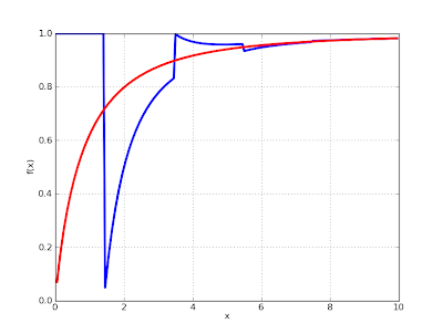
It's instructive to visualize the optimal truncations of an asymptotic series compared to the exact solution. Notice how, for an alternating series like this, the truncations alternate between over- and undershooting:
def optimal_asymp(z):
    u = -4/(z**2)
    term_prev = inf
    s = 0.0
    for k in range(30):
        term = rf(0.5,k)*rf(1,k)*rf(1,k)*u**k/fac(k)
        if abs(term) < abs(term_prev):
            s += term
            term_prev = term
        else:
            break
    return s

def exact(z):
    u = -4/(z**2)
    return hyper([0.5,1,1],[],u)

mp.dps = 10
plot([optimal_asymp, exact], [0,10])

The catch with this feature? Computing the Borel regularization involves evaluating (nested) numerical integrals with a hypergeometric function in the integrand. Except for special parameters (where degree reductions happen internally -- the Ci series above happens to be such a case), it's not very fast.
Optional consistency with Mathematica
I often try to follow Mathematica's conventions regarding limits, special values and branch cuts of special functions. This simplifies testing (I can directly compare values with Mathematica), and usually Mathematica's conventions seem well-reasoned.
There are exceptions, however. One such exception concerns Mathematica's interpretation of 2F1(a,b,c,z) for b = c a negative integer. Mathematica interprets this as a polynomial, which doesn't make much sense since the denominator of the zero term is zero. It's not even consistent with how Mathematica evaluates this function for a symbolic variable:
In[3]:= Hypergeometric2F1[3,-2,-2,2]

Out[3]= 31

In[4]:= Hypergeometric2F1[3,b,b,2]

Out[4]= -1
Maybe there is a good reason for doing what Mathematica does, but it's at the very least not documented anywhere. I've now changed mpmath to instead interpret the two parameters as eliminating each other and giving a 1F0 function (which is what Mathematica does for a generic value). The Mathematica-compatible value can be recovered by explicitly disabling parameter elimination:
>>> mp.pretty = True
>>>
>>> hyp2f1(3,-2,-2,2)
-1.0
>>> hyp2f1(3,-2,-2,2,eliminate=False)
31.0
On a related note, I've fixed the Meijer G-function to switch between its z and 1/z forms automatically to follow Mathematica's definition of the function. This introduces discontinuities in the function for certain orders. The user can explicitly choose which form to use (so as to obtain a continuous function) with series=1 or series=2.
Internal reorganization
In a long overdue change, I've moved many of the modules in mpmath into subdirectories. The multiprecision library code is now located in mpmath/libmp; special functions are in mpmath/functions, calculus routines are in mpmath/calculus, and routines for matrices and linear algebra are in mpmath/matrices.
This shouldn't affect any documented interfaces, but it will break external code that directly uses mpmath internal functions. The mpmath interfaces in SymPy and Sage will need some editing for the next version update. The breakage should be straightforward to fix (mostly just a matter of changing imports).
Since the next version of mpmath is definitely going to break some code, I might use the opportunity to do some other cosmetic interface changes as well. Ideally, after the next version, the interface will be stable until and beyond mpmath 1.0 (whenever that happens). But the version number is still at 0.x for a reason -- no compatibility guarantees.
1 comment:
Which versions of mpmath are your referring to in this article?
Post a Comment