Monday, June 21, 2010

Incomplete elliptic integrals complete

I'm very happy to finally have implemented incomplete elliptic integrals in mpmath (they were probably the most-requested missing special functions). Now mpmath can compute the three classical (Legendre) elliptic integrals F(φ, m), E(φ, m), Π(n, φ, m) as well Carlson's symmetric integrals RF, RC, RJ, RD, RG. Previously only the complete integrals K(m) and E(m) were available.

The functions are called, respectively, ellipf, ellipe, ellippi, elliprf, elliprc, elliprj, elliprd, elliprg, although this could change before the release. For the code, see r1162, r1166 and adjacent commits; documentation is available in the elliptic functions section.

This work was possible thanks to the support of NSF grant DMS-0757627, gratefully acknowledged.

Elliptic integral basics


What are elliptic integrals and why are they important? As the name suggests, they are related to ellipses. Given an ellipse of width 2a and height 2b, i.e. satisfying


or using an angular coordinate θ


the arc length along the ellipse from θ = 0 to θ = φ is given by


where m = 1-(a/b)^2 is the so-called elliptic parameter.

Here are some plots of half-ellipses of various proportions, and the corresponding arc lengths:

a = 1
b1 = 0.1; f1 = lambda x: b1*sqrt(1 - (x/a)**2)
b2 = 0.6; f2 = lambda x: b2*sqrt(1 - (x/a)**2)
b3 = 1.0; f3 = lambda x: b3*sqrt(1 - (x/a)**2)
b4 = 2.0; f4 = lambda x: b4*sqrt(1 - (x/a)**2)
plot([f1,f2,f3,f4], [-1,1])

g1 = lambda phi: b1*ellipe(phi, 1-(a/b1)**2)
g2 = lambda phi: b2*ellipe(phi, 1-(a/b2)**2)
g3 = lambda phi: b3*ellipe(phi, 1-(a/b3)**2)
g4 = lambda phi: b4*ellipe(phi, 1-(a/b4)**2)
plot([g1,g2,g3,g4], [0,pi])


The preceding formulas are sometimes seen with a and b switched, which simply corresponds to transposing x and y as the reference axis (above, the integration is assumed to start on the x axis). One can readily confirm that E(φ, m) satisfies obvious geometric symmetries:


>>> a = 0.5
>>> b = 0.25
>>> m1 = 1-(a/b)**2
>>> m2 = 1-(b/a)**2
>>> b*ellipe(pi/2,m1) # Arc length of quarter-ellipse
0.6055280137842297624017815
>>> a*ellipe(pi/2,m2)
0.6055280137842297624017815
>>> a*ellipe(pi/4,m2) + b*ellipe(pi/4,m1)
0.6055280137842297624017815
>>> a*ellipe(pi/3,m2) + b*ellipe(pi/6,m1)
0.6055280137842297624017815


Elliptic integrals have countless uses in geometry and physics, and even in pure mathematics. They are related to Jacobi elliptic functions (already available in mpmath), which essentially are inverse functions of elliptic integrals:


>>> m = 0.5
>>> sn = ellipfun('sn')
>>> ellipf(asin(sn('0.65', m)), m)
0.65


More information about elliptic integrals can be found in DLMF Chapter 19.

Implementation


Implementing incomplete elliptic integrals properly is fairly complicated. When people have asked for them in the past, I just suggested using numerical integration. This works quite well most of the time, but it's inefficient (and possibly gives poor accuracy) at high precision, for large arguments, or near singularities. Another approach — computing incomplete integrals from Appell hypergeometric functions (available in mpmath) — basically has the same drawbacks.

The numerically conscious way to compute elliptic integrals is to firstly exploit symmetries to obtain a small standard domain, and then using transformation formulas to reduce the magnitude of the arguments until the first few terms of the hypergeometric series give full accuracy (the arithmetic-geometric mean for the complete integrals, which leads to some of the fastest ways to compute π, is a special case of this process).

The transformations for Legendre's integrals are known as Landen's transformations. A more modern alternative, that I've chosen to use, is to represent Legendre's integrals in terms of Carlson's symmetric integrals which have much simpler structure. Although Carlson's integrals are mainly intended for internal use, I've exposed them as top-level functions since it wasn't much extra work and some users may well find them useful. (Carlson's forms seem to become increasingly standard.)

Carlson's paper is very readable and provides almost complete descriptions of the algorithms, including error bounds, which helped my implementation work tremendously. The error bounds are not rigorous in all cases, but good enough most of the time. Unfortunately, there are many special cases to consider, and Carlson does not address all of them explicitly, so putting it all together nevertheless involved a bit of work (and there are still some minor issues to fix).

Complex branch structure


One major issue is how to define the elliptic integrals for complex (or in some places, negative) parameters. Because the integrands defining Legendre's elliptic integrals involve square roots of periodic functions, they have very complicated branch structure. I have chosen the periodic extension of the branches resulting naturally from use of the Carlson forms on -π/2 < Re(z) < π/2. I believe this is equivalent to choosing the principal-branch square root in the integrand and integrating along a path where the principal branch is continuous.

For example, consider E(φ, 3+4i). The integrand (with the principal square root, as computed by sqrt) and the elliptic integral computed by ellipe are plotted below:

>>> cplot(lambda z: sqrt(1-(3+4j)*sin(z)**2), points=50000)


>>> cplot(lambda z: ellipe(z, 3+4j), points=50000)


It can be seen that the cuts have the same shape in both images (the branch points are necessarily the same). As the following figure shows, if we are to integrate from z = 0 to z = -2+4i (X), a straight path (black) will be bad as it crosses a branch cut (O). However, the modified path (blue) avoiding the branch cut by passing through z = -2 is fine:


We can confirm this with numerical integration:

>>> ellipe(-2+4j, 3+4j)
(36.45544164923053561755261 + 49.28080768743760310823023j)
>>> quad(lambda z: sqrt(1-(3+4j)*sin(z)**2), [0,-2+4j])
(19.65109997738606076596704 + 46.63216059660102110020723j)
>>> quad(lambda z: sqrt(1-(3+4j)*sin(z)**2), [0,-2,-2+4j])
(36.45544164923053561755261 + 49.28080768743760310823023j)


Unfortunately, Mathematica doesn't use quite the same branch cuts for its elliptic integrals. I don't have Mathematica available to create a plot for comparison purposes, but I think it basically uses vertical cuts instead of the curvilinear cuts seen in the images above. There are probably good reasons for doing this, presumably that it simplifies symbolic definite integration, although it seems to complicate the evaluation and formulaic representation of the functions. It would perhaps be good to support both conventions.

As far as the symmetric functions are concerned, they have the nice property that although they involve non-principal square roots (chosen so as to be continuous along the real line), Carlson's algorithm gives the continuous branch automatically. For example, if we consider the first function


with x = i-1, y = i, z = 0, then as the following plot shows, the principal branch of the integrand has a discontinuity at t = 1/2:


>>> x,y,z = j-1,j,0
>>> f = lambda t: 1/sqrt((t+x)*(t+y)*(t+z))
>>> plot(f, [0,3])


To obtain the correct integrand, we switch to the negative square root on the left of the discontinuity (the positive sign should be used on the right because, for continuity with real parameters, we want the principal square root as t → +∞):

>>> g = lambda t: f(t) if t >= 0.5 else -f(t)
>>> plot(g, [0,3])


A quick test shows that f is wrong and g is right:


>>> extradps(25)(quad)(f, [0,inf])/2
(1.110136183412179775397387 - 0.04278194644898641314159222j)
>>> extradps(25)(quad)(g, [0,inf])/2
(0.7961258658423391329305694 - 1.213856669836495986430094j)
>>> elliprf(x,y,z)
(0.7961258658423391329305694 - 1.213856669836495986430094j)


In summary, branch cuts of special functions are a tricky business, and standards don't always exist, so both developers and users need to be careful working with them.

Tuesday, June 15, 2010

Assorted special functions update

Over the week-and-a-half since the last blog update, I've gotten a bunch more work done on special functions in mpmath.

Function plots in the documentation


I have started adding graphics of special functions to the documentation. So far, I've done most of the Bessel-type functions and orthogonal polynomials. Many more to come!

Example screenshot (see the Bessel functions page):


New inhomogeneous Bessel functions


There exists a large number of lesser-known special functions which are essentially variations of Bessel functions. These include functions which solve the generalized (inhomogeneous) Bessel differential equation


with some specific right-hand side g(z). New additions to mpmath in this category are the Anger function (angerj()), Weber function (webere()), and Lommel functions (lommels1(), lommels2()). See commits here and here.

More information about Anger-Weber functions and Lommel functions can be found in the DLMF.

In the near future, I will probably further improve the implementations of the main Bessel functions. The Bessel functions are mostly implemented as generic hypergeometric functions, but the standard cases can be tuned a great deal with special-purpose code.

Airy functions and related functions


The Airy functions Ai and Bi have been present for quite some time in mpmath. In a recent commit, I have rewritten them for improved rigor and better performance at high precision. There are also some new features, such as the ability to evaluate derivatives or iterated integrals of arbitrary order.

Derivatives:

>>> from mpmath import *
>>> mp.dps = 25; mp.pretty = True
>>> airyai(1.5, derivative=5)
0.211387453153454489799743
>>> diff(airyai, 1.5, 5)
0.211387453153454489799743
>>> airyai(1.5, derivative=100)
-6.480220187791312407132043e+49
>>> airybi(0, derivative=1000)
3.754976097101270163249629e+854
>>> airybi(0, derivative=1001)
0.0
>>> airybi(0, derivative=1002)
3.756228172694934424506624e+856


Integrals:

>>> airyai(5, derivative=-1)
0.3332875903059178794866562
>>> quad(airyai, [0,5])
0.3332875903059178794866562
>>> airyai(-100000, derivative=-1)
-0.6665753658794626398413214


Also, functions for computing the zeros of Ai and Bi (and the first derivatives) have been added:

>>> airyaizero(1)
-2.338107410459767038489197
>>> airyaizero(2)
-4.087949444130970616636989
>>> airybizero(1)
-1.17371322270912792491998
>>> airybizero(1, derivative=1)
-2.294439682614123246622459
>>> airybizero(1, derivative=1, complex=True)
(0.2149470745374305676088329 + 1.100600143302797880647194j)
>>> airybizero(10000)
-1304.584974702601410702964
>>> airybizero(10000, complex=True)
(652.3059222438076432024695 + 1129.846189716375208308414j)


I have also implemented two new functions related to Airy functions: the Scorer functions Gi and Hi. These are available as scorergi() and scorerhi() respectively.

Here are two plots of the Gi-function, which can also be seen in the documentation:


Interval gamma functions


The interval arithmetic context now implements gamma, rgamma (reciprocal gamma function), factorial as well as loggamma for real as well as complex arguments (commit). For example:

>>> iv.dps = 10
>>> iv.gamma('50.3')
[1.96282982095908e+63, 1.96282982457481e+63]
>>> iv.gamma(iv.mpc('2.7','5.9'))
([0.00269836072064322, 0.00269836072271801] +
[0.0120124287790304, 0.0120124287810768]*j)


As a "practical" example, consider evaluating the Riemann-Siegel theta function which involves computing the difference of two log-gamma functions. For input with a large real part, the imaginary part in the result suffers from massive cancellation and may end up with the wrong sign:

>>> mp.dps = 15
>>> mp.siegeltheta(10**50 + 0.25j)
(5.61456887916465e+51 - 0.143091235731175j)
>>> mp.dps = 10; nprint(mp.siegeltheta(10**50 + 0.25j).imag)
-0.143091
>>> mp.dps = 100; nprint(mp.siegeltheta(10**50 + 0.25j).imag)
14.1614


With interval arithmetic, the sign uncertainty is reflected in the output:

>>> iv.dps = 15
>>> iv.siegeltheta(10**50 + 0.25j)
([5.6145688791646467648e+51, 5.6145688791646474294e+51] +
[-5.0706024009129187319e+30, 5.070602400912917606e+30]*j)
>>> iv.dps = 50
>>> iv.siegeltheta(10**50 + 0.25j)
([5614568879164647368060513633451316140100495086670736.0, 5614568879164647368060
513633451316140100495086670744.0] +
[14.1613521236438249782320715810808676610440
8814838558203, 14.16147419395632497823207158108086766104408814838560341]*j)


As another example, consider evaluating the gamma function of a huge argument. The digits in the answer may be "wrong" because the input is converted from decimal to binary, and the gamma function is sensitive to the input being perturbed:

>>> mp.dps = 15
>>> mp.gamma('123456789012345.1')
6.11544992055093e+1686076589184486
>>> mp.dps = 30
>>> mp.gamma('123456789012345.1')
7.49032018540342193592769680745e+1686076589184486
>>> mp.dps = 60
>>> mp.gamma('123456789012345.1')
7.49032018540342058679709881225047421518964527875047787194339e+1686076589184486


With interval arithmetic, the uncertainty in the input is propagated correctly:

>>> iv.dps = 15
>>> iv.nprint(iv.gamma('123456789012345.1'), mode='diff')
[6.11545e+1686076589184486, 1.01533e+1686076589184487]
>>> iv.dps = 30
>>> iv.nprint(iv.gamma('123456789012345.1'), 20, mode='diff')
7.4903201854034[185631, 219359]e+1686076589184486
>>> iv.dps = 60
>>> iv.nprint(iv.gamma('123456789012345.1'), 50, mode='diff')
7.49032018540342058679709881225047421518964527[60898, 87505]e+1686076589184486


Rewritten Lambert W function


Lastly, the Lambert W function has received a much-needed rewrite (commit) mainly to improve evaluation very close to the branch cut along the negative axis and particularly near the branch point at -1/e for the k = -1, 0, 1 branches.

With the previous implementation, results were frequently inaccurate or ended up on the wrong branch in this region. Here are some hard cases that now work perfectly:


>>> mp.dps = 1000
>>> x = -1/e + mpf('1e-900')
>>> y = -1/e - mpf('1e-900')
>>> z = -1/e + mpf('1e-900')*1j
>>> w = -1/e - mpf('1e-900')*1j
>>> mp.dps = 25
>>> lambertw(x,0); lambertw(y,0); lambertw(z,0); lambertw(w,0)
-1.0
(-1.0 + 2.331643981597124203363536e-450j)
(-1.0 + 1.648721270700128146848651e-450j)
(-1.0 - 1.648721270700128146848651e-450j)
>>> lambertw(x,1); lambertw(y,1); lambertw(z,1); lambertw(w,1)
(-3.088843015613043855957087 + 7.461489285654254556906117j)
(-1.0 + 1.648721270700128146848651e-450j)
>>> lambertw(x,-1); lambertw(y,-1); lambertw(z,-1); lambertw(w,-1)
-1.0
(-1.0 - 2.331643981597124203363536e-450j)
(-1.0 - 1.648721270700128146848651e-450j)
(-3.088843015613043855957087 - 7.461489285654254556906117j)


To finish this post, I present the following Mathematica bug:


remote1:frejohl:[~]$ math
Mathematica 7.0 for Linux x86 (32-bit)
Copyright 1988-2008 Wolfram Research, Inc.

In[1]:= Im[LambertW[0,-1/E-10^(-900)]]

Out[1]= 0

Sunday, June 6, 2010

Announcing mpmath 0.15

I'm happy to announce the release of mpmath 0.15!

This should've happened earlier, but I was obstructed by other obligations (in particular, finishing my master's thesis). The good news is that I will be working full-time on special functions in mpmath and Sage again this summer thanks to sponsorship provided by William Stein (with money from an NSF grant). I will also come to Sage Days 23 (July 5-9, Leiden, the Netherlands) and Sage Days 24 (July 17-22, Linz, Austria) which should be as fun as SD15.

What's new in mpmath 0.15? As usual, the details can be found in the CHANGES file and the list of commits. Most major changes were covered in detail in previous blog posts, so I will first of all simply link to those posts along with short summaries:

Speedups of elementary functions - cos, sin, atan, cosh, sinh, exp and all derived functions are now faster. Of particular note, trigonometric functions use an asymptotically faster algorithm (all elementary functions have similar asymptotic performance now).

A new gamma function implementation
- the gamma function and log-gamma functions have been rewritten scratch, using faster algorithms and code optimizations. The new versions are uniformly faster than the old ones, and tens or hundreds of times faster in many important situations. They are also more accurate in some special cases (near singularities, for complex arguments with extremely small real part, ...).

Numerical multidimensional infinite series - nsum() can now evaluate series (finite or infinite) in any number of dimensions

Computing large zeta zeros with mpmath - Juan Arias de Reyna has implemented code for computing the nth zero of the Riemann zeta function on the critical line for arbitrarily large n. On a related note, the Riemann zeta function code has been optimized (mostly through elimination of low-level overhead) to speed up such computations.

Hypergeneralization - generalized 2D hypergeometric series, bilateral hypergeometric series and some q-analogs (q-Pochhammer symbol, q-factorial, q-gamma function, q-hypergeometric series) have been implemented.

In addition, there are many changes that I haven't had time to blog about yet. I will now write briefly about some of these:

Elliptic functions


The support for working with elliptic functions has been improved. Instead of just the standard three, all 12 Jacobi elliptic functions are now available via ellipfun, e.g. the cd-function:

>>> from mpmath import *
>>> mp.dps = 25; mp.pretty = True
>>> ellipfun('cd', 3.5, 0.5)
-0.9891101840595543931308394
>>> cd = ellipfun('cd')
>>> cd(3.5, 0.5)
-0.9891101840595543931308394

Functions qfrom(), qbarfrom(), mfrom(), kfrom(), taufrom() have also been added to convert between the various forms of arguments to elliptic functions (nomes (two definitions), parameters, moduli, half-period ratios). If you're like me and never can remember such formulas, let alone avoid messing up when trying to apply them, this can be quite convenient. Some functions (in particular, ellipfun also support direct choice of convention using keyword arguments):


>>> ellipfun('sn',2,1+1j) # default is m
(1.333680690847080418060154 - 0.2084318767795699518406447j)
>>> ellipfun('sn',2,q=qfrom(m=1+1j))
(1.333680690847080418060154 - 0.2084318767795699518406447j)
>>> ellipfun('sn',2,k=kfrom(m=1+1j))
(1.333680690847080418060154 - 0.2084318767795699518406447j)
>>> ellipfun('sn',2,tau=taufrom(m=1+1j))
(1.333680690847080418060154 - 0.2084318767795699518406447j)


Another new function is the Klein j-invariant (or rather, the "absolute invariant" or "J-function" which differs by a constant factor, and also is the normalization used by Mathematica). A nice application is to compute the Laurent series expansion in terms of the (number-theoretic) nome, giving a famous integer sequence:

>>> mp.dps = 15
>>> taylor(lambda q: 1728*q*kleinj(qbar=q), 0, 5, singular=True)
[1.0, 744.0, 196884.0, 21493760.0, 864299970.0, 20245856256.0]


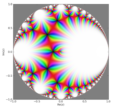
The J-function also looks pretty when plotted, here as a function of the number-theoretic nome within the unit circle:

fp.cplot(lambda q: fp.kleinj(qbar=q), [-1,1], [-1,1], points=400000)


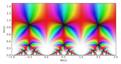
As a function of the half-period ratio τ, defined in the upper half-plane:
fp.cplot(lambda t: fp.kleinj(tau=t), [-1,2], [0,1.5], points=100000)


Complex interval arithmetic


The support for interval arithmetic has been extended; there is also a new interface for intervals. It is no longer possible to call mpmath.exp etc. directly with interval arguments; instead all interval arithmetic has been moved to a separate context object called iv (similar to the separate interface for working with Python float/complex in mpmath). For example:

>>> iv.dps = 5; iv.pretty = True
>>> iv.mpf(1)/3
[0.3333330154, 0.3333334923]
>>> iv.sin(1)
[0.8414707184, 0.8414716721]
>>> iv.sin([1,2])
[0.8414707184, 1.0]
>>> iv.sin([1,3])
[0.141119957, 1.0]

The interface change was done to simplify the implementation; separating out interval arithmetic also helps avoid inadvertent mixing of interval and non-interval arithmetic.

There is also some support for complex interval arithmetic, including some elementary functions (exp, log, cos, sin, power).


>>> iv.mpc('1.3','1.4') ** 2
([-0.2700066566, -0.2699956894] + [3.639995575, 3.640010834]*j)
>>> iv.mpc('1.3','1.4') ** iv.mpc('1.2','-0.7')
([3.329280853, 3.329311371] + [1.967472076, 1.967498779]*j)
>>> iv.dps = 25
>>> iv.mpc('1.3','1.4') ** 2
([-0.270000000000000000000000061005, -0.269999999999999999999999912371] +
[3.63999999999999999999999988419, 3.64000000000000000000000009099]*j)
>>> mp.cos(2+3j)
(-4.189625690968807230132555 - 9.109227893755336597979197j)
>>> iv.cos(2+3j)
([-4.18962569096880723013255508975, -4.18962569096880723013255498635] +
[-9.1092278937553365979791973006, -9.10922789375533659797919709381]*j)


Verifying Euler's identity:

>>> iv.dps = 5
>>> iv.exp(1j * iv.pi)
([-1.0, -0.9999990463] + [-1.279517164e-6, 2.535183739e-6]*j)
>>> iv.dps = 25
>>> iv.exp(1j * iv.pi)
([-1.0, -0.999999999999999999999999987075] +
[-1.8806274411915714063022730148e-26, 3.28925138726485156164403137746e-26]*j)

Rigorous complex linear algebra:

>>> iv.dps = 15
>>> A = iv.matrix([[2,-2,1],[1,0,2],[1,1,2]])
>>> b = iv.matrix([1,2+2j,5])
>>> iv.lu_solve(A,b)
[ ([4.0, 4.0] + [-3.3333333333333333339, -3.333333333333333333]*j)]
[([3.0, 3.0] + [-2.0000000000000000004, -1.9999999999999999998]*j)]
[ ([-1.0, -1.0] + [2.6666666666666666665, 2.666666666666666667]*j)]
>>> A*iv.lu_solve(A,b)
[([1.0, 1.0] + [-8.8817841970012523234e-16, 1.7763568394002504647e-15]*j)]
[ ([2.0, 2.0] + [1.9999999999999995559, 2.0000000000000008882]*j)]
[([5.0, 5.0] + [-8.8817841970012523234e-16, 1.7763568394002504647e-15]*j)]


Partial derivatives


This is rather simple, but very convenient. diff can now compute partial derivatives of arbitrary order for multivariable functions. For example, a first derivative with respect to the second argument:

>>> diff(lambda x,y: 3*x*y + 2*y - x, (0.25, 0.5), (0,1))
2.75

The first derivative with respect to both x and y:

>>> diff(lambda x,y: 3*x*y + 2*y - x, (0.25, 0.5), (1,1))
3.0


Second derivative with respect to a parameter of a hypergeometric function 2F1(a,b,c,z); tenth derivative with respect to the argument; first derivative with respect to two parameters and fourth derivative with respect to the argument:

>>> diff(hyp2f1, (1,2,3,0.5), (0,0,2,0))
0.2306514802159766624657329
>>> diff(hyp2f1, (1,2,3,0.5), (0,0,0,10))
672869392.1810426015397572
>>> diff(hyp2f1, (1,2,3,0.5), (1,0,1,4))
-585.1335939248098118753126


That's it for now. Stay tuned for many new features in the near future!