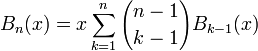
In particular, Bn(1) is the nth Bell number, which has combinatorial significance as the number of partitions of a set with n elements.
Instead of using the recurrence formula above, I implemented an approximate formula (discussed below) to provide fast approximate evaluation. So it is for example possible to do:
>>> from mpmath import *
>>> mp.dps = 30
>>> print bell(100000)
1.04339424254293899845402468388e+364471
This algorithms turns out to work well for exact evaluation at integer arguments, by setting the precision large enough, e.g. like this:
>>> from mpmath import *
>>> from mpmath.functions import funcwrapper
>>>
>>> @funcwrapper
... def bellexact(n,x=1):
...     mp.prec = 20
...     size = int(log(bell(n,x),2))+10
...     mp.prec = size
...     return int(bell(n,x)+0.5)
...
>>> bellexact(100)
47585391276764833658790768841387207826363669686825611466616334637559114
622672724044217756306953557882560751L
>>>
>>> bellexact(50)
185724268771078270438257767181908917499221852770L
>>> bellexact(40,40)
5288533501514377257070614176831982123270530650242136500078910824523240L
I did a bit of benchmarking for computing large Bell numbers Bn, and this approach appears to be much faster than what other systems use. Below are my timings for SymPy, GAP, Mathematica, and mpmath. (Note: as I do not have a personal Mathematica license, I ran it remotely on a different system, which based on a comparison of integer multiplication speed is 10-20% faster than my own laptop.)
      n        SymPy      GAP   Mathematica    mpmath
    100      0.007 s      0 s       0.005 s   0.012 s
    1000       8.9 s   0.78 s        0.32 s    0.30 s
    3000           -     67 s          12 s     3.6 s
    10000          -        -         396 s      76 s
From what I've read, Bell numbers have some interesting number-theoretical properties such as Touchard's congruence, so this could potentially be useful to someone. (Interestingly, I wonder if Touchard's congruence could be turned into an even faster modular algorithm for Bell numbers, similar to David Harvey's algorithm for Bernoulli numbers.)
The formula I implemented for the Bell polynomials is the infinite series
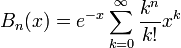
which is known by the name Dobinski's formula.
As a side note, I implemented this series using a piece of experimental new summation code designed to ensure full accuracy in spite of cancellation. For example, the following evaluation involves alternating terms of magnitude over 10400; the internal precision is automatically set to over 400 digits to provide the requested 15 digits:
>>> mp.dps = 15
>>> print bell(10,-1000)
9.55744142784509e+29
I'll probably be working more this summer on implementing similar methods for several mpmath functions that are currently implemented somewhat less robustly (more on that some other time).
One interesting aspect of Dobinski's formula is that it generalizes to arbitrary complex values for n, not just integers. I always prefer to implement functions for the most general possible arguments (and will sometimes hesitate to implement a function if I can only do it for a special case). Generalization is extremely useful: extending functions defined on the integers to the reals permits the use of differentiation, continuous optimization algorithms, etc. Extending further to the complex numbers allows for contour integration. Curiously, Mathematica does not seem to do this for its BellB function.
Unfortunately, there is a difficulty in implementing Dobinski's formula for general n: the 0th term is singular unless n is a nonnegative real number. Removing the term completely breaks compatibility with the standard definition of the Bell polynomials for n = 0. Keeping it either makes the series undefined, or at best renders the function discontinuous at the single point n = 0 which is certainly not desirable. As a workaround, I changed the formula to
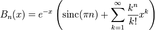
The sinc term is continuous (analytic), and zero when n is an integer except when n = 0, so it solves all problems. The sinc function has no connection to Bell polynomials whatsoever as far as I know, but it is the simplest possible "patch" I can think of.
Voila, we now get a smooth transition between for example B0(x) = 0 and B1(x) = x:
>>> f = lambda k: (lambda x: bell(k,x))
>>> plot([f(k) for k in linspace(0,1,5)], [-2,3])
It also becomes possible to e.g. compute a Taylor series of B seen as a function of n, using either a step sum or complex integration for the derivatives:
>>> nprint(chop(taylor(lambda n: bell(n,1), 0, 5, method='step')))
[1.0, 0.222119, -0.504269, 3.32909e-2, 0.307601, 2.09191e-3]
>>> nprint(chop(taylor(lambda n: bell(n,1), 0, 5, method='quad')))
[1.0, 0.222119, -0.504269, 3.32909e-2, 0.307601]
We can for example use the Taylor expansion around n = 0 to evaluate the Bell polynomial with n = 1 (not really practical for anything, but a beautiful example of the power of analysis):
>>> print polyval(taylor(lambda n: bell(n,3), 0, 5)[::-1], 1)
2.9949024096858
>>> print polyval(taylor(lambda n: bell(n,3), 0, 10)[::-1], 1)
2.99998868106305
>>> print polyval(taylor(lambda n: bell(n,3), 0, 15)[::-1], 1)
2.99999998751065
>>> print polyval(taylor(lambda n: bell(n,3), 0, 25)[::-1], 1)
3.0
>>> print bell(1,3)
3.0
Finally, I also implemented the raw series

as a separate function, because it seems like it could be useful in its own right. Unfortunately, this function does not appear to have a standardized notation. For certain special values, it reduces to a Bell polynomial times an exponential function; an incomplete gamma function; or a generalized hypergeometric function. It is also related to the Poisson distribution. Other than that, I have not found much information about it. Does this function have a name? I named it polyexp in mpmath, because it can be seen as an exponential analog of the polylogarithm.
As a function of s, it is an L-series, and shows interesting, highly chaotic behavior in the complex plane:
>>> mp.dps = 5
>>> cplot(lambda s: polyexp(s,1), [-20,20],[0,60], points=50000)
>>> plot(lambda s: polyexp(s*j,1), [0,60])

