I must first apologize for taking over three months since the last release, but there are many new features that hopefully will make the delay worthwhile. In this blog post, I will present most of the new features in some detail. There are many smaller changes that I won't mention; see the changelog for a more complete list.
This post will contain many doctest-type examples run in the Python interactive interpreter. I should note that they will assume that mpmath has been imported as follows:
>>> from mpmath import *
Now, in no particular order:
More documentation
Most functions in mpmath now have extensive docstrings, with many code examples. The examples cover a lot of interesting mathematics, so the documentation might even have some educational value! The Sphinx-generated HTML documentation now displays properly Latex-rendered math formulas, so it looks much better (and is easier to read) too. You can view the HTML documentation here.
Speed improvements
Mpmath 0.11 is significantly faster than 0.10, due to a combination of optimizations to core functions in mpmath and improved integration with gmpy. Version 1.04 of gmpy, which is not released at the time of writing but should be available any day now, makes the mpmath unit tests run about 30% faster compared to 1.03, due to optimizations implemented by Case Vanhorsen and Mario Pernici (many thanks).
As usual, I must stress that mpmath is a pure-Python library, and gmpy is optional for better performance. That said, using the unit tests as a benchmark, mpmath is now more than twice as fast in gmpy mode than in pure-Python mode, so anyone who is interested in doing serious calculations should install gmpy. (At high precision, gmpy-mode is orders of magnitude faster.)
The following particular example (integrating sqrt(x) over [1,2]) is 2.7x faster in mpmath 0.11 than in 0.10, due to a combination of the aforementioned general improvements and optimizations of numerical quadrature:
    >>> import sympy.mpmath as m   # mpmath 0.10
    >>> timing(m.quad, m.sqrt, [1, 2])
    0.0046395002716825753
    >>> timing(quad, sqrt, [1, 2])  # mpmath 0.11
    0.0017537424449196592
On the algorihmic side, Mario has written new code for exp and log at high precision. Above a couple of thousand digits, the natural logarithm is now calculated using the Sasaki-Kanada formula, which expresses the logarithm as the arithmetic-geometric mean of two Jacobi theta functions. The exponential function in turn is computed from the natural logarithm using a high-order Newton method. At 100,000 digits, this is about 3x faster than the old code, with either log or exp taking about 3 seconds on my computer:
    >>> timing(ln, 1.2345, dps=10**5)
    3.1008502477270152
    >>> timing(exp, 1.2345, dps=10**5)
    3.1638269668351704
It needs to be pointed out that the speed of these algorithms depends fundamentally on the asymptotically fast arithmetic provided by gmpy. The speedup in pure-Python mode is much smaller.
Special functions
A major change in 0.11 is the support for Jacobi theta and elliptic functions, which have been rewritten from scratch by Mario. They are now very fast, and work for almost all possible arguments, even very close to the boundary of analyticity at |q| = 1:
    >>> mp.dps = 30
    >>> print jtheta(3, 1, mpf(6)/10 - mpf(10)**(-6) - mpf(8)/10*j)
    (32.0031009628901652627099524204 + 16.6153027998236087899308920259j)
There is also a new function djtheta that computes nth derivatives of Jacobi theta functions, for arbitrary n.
Many other functions have been added. Mpmath now provides Bessel Y, I and K functions (it previously only provided the J function), as well as Hankel functions. These were implemented due to requests on the scipy mailing lists. Other new functions include the sinc function, polylogarithms, the Dirichlet eta function (alternating zeta function), the inverse error function, and the generalized incomplete gamma function. Improvements include faster evaluation of Stieltjes constants, trigonometric integrals, and the exponential integral for large arguments.
Some examples that now work:
    >>> mp.dps = 30

    >>> print polylog(2,j); print j*catalan - pi**2/48
    (-0.205616758356028304559051895831 + 0.915965594177219015054603514932j)
    (-0.205616758356028304559051895831 + 0.915965594177219015054603514932j)

    >>> print quadosc(sinc, [-inf, inf], omega=1)
    3.14159265358979323846264338328

    >>> print bessely(2.5, pi)
    -0.313326485870232269369501914258
    >>> print hankel1(1, 0.5)
    (0.242268457674873886383954576142 - 1.47147239267024306918858463532j)

    >>> print identify(altzeta(7), ['zeta(7)'])
    ((63/64)*zeta(7))

    >>> print stieltjes(100)
    -425340157170802696.231443851973

    >>> print erf(erfinv('0.99995'))
    0.99995

    >>> print ci(10**6)
    -0.000000349994438922720492637592474167
    >>> print ei(10**6)
    3.03321843002355079616691658126e+434288

    >>> print gammainc(3.5,2,10); print quad(lambda t: t**2.5/exp(t), [2,10])
    2.57296399554551364489515478158
    2.57296399554551364489515478158
A few more combinatorial functions were also added: Fibonacci numbers, double factorials, superfactorials and hyperfactorials. The implementation is not really designed for computing large exact values of these functions. Rather, it is intended for computing large approximate values, and this is fast because asymptotic expansions are used.
    >>> mp.dps = 15
    >>> for f in [fib, fac2, superfac, hyperfac]:
    ...     print f(5)
    ...
    5.0
    15.0
    34560.0
    86400000.0

    >>> for f in [fib, fac2, superfac, hyperfac]:
    ...     print f(10**6)
    ...
    1.95328212870776e+208987
    1.01770845550781e+2782856
    6.92872856133331e+2674285103370
    6.23843686069242e+2891429379524

    >>> for f in [fib, fac2, superfac, hyperfac]:
    ...     print f(4+2j)
    ...
    (-8.23269197092811 + 16.8506564651585j)
    (-5510415655129.54 + 78867063149796.4j)
    (2.39042329112716 + 10.8983226702567j)
    (140.651495550631 + 109.654202164718j)
Note that these functions support arbitrary real and complex arguments. Why is this useful? For one thing, the defining functional equations (e.g. fib(n+1) = fib(n) + fib(n-1)) extend to the complex plane, which is neat. More practically, it allows one to do differentiation, contour integration, etc, which can be very useful. For example, this permits the Euler-Maclaurin formula to be applied to sums containing Fibonacci numbers, double factorials, superfactorials or hyperfactorials.
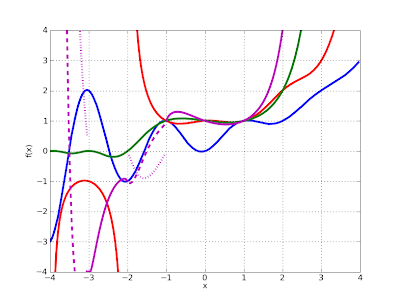
Here is a plot of the four functions on the real line (Fibonacci in blue, double factorial in red, superfactorial in green, hyperfactorial in purple):
>>> plot([fib, fac2, superfac, hyperfac], [-4, 4], [-4, 4])

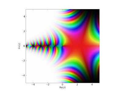
For those interested, the generalization of superfactorials and hyperfactorials uses the Barnes G-function, which itself is now available as barnesg. It can be visualized in the complex plane as follows (warning: somewhat sluggish):
    >>> mp.dps = 5
    >>> cplot(barnesg, points=50000)

High-precision ODE solver
Since earlier, mpmath contains a basic nonadaptive RK4 solver for ordinary differential equations (ODEs). This is fine for many purposes, but limited to low precision (3-5 digits), and the user must supply the evaluation points.
The new solver is based on Taylor series, and works with arbitrarily high degrees. This means that high accuracy is attainable relatively cheaply. Also importantly, the computed Taylor series are natural interpolants, so once the ODE has been solved on an interval [a, b], the solution function can be evaluated anywhere on [a, b] in a fraction of a second by a simple call to polyval. This is handled automatically.
As an example, let's try to solve y''(x) = cos(2x) y(x) with initial conditions y(0) = 1, y'(0) = 0. This is an instance of the Mathieu differential equation. Mpmath does not yet implement Mathieu functions, so this is a nice application; the generic ODE solver could be used to verify a future specialized implementation, to generate a full-accuracy machine precision approximant (for "real world" use), etc.
The solver works with first-order ODEs, so we rewrite the equation as a first-order, two-dimensional system by adding y' as a variable. odefun takes a function that evaluates the derivatives, the initial x point, and the initial vector. It returns a function that evaluates the solution; in this case, we get both the solution function and its derivative:
    >>> mp.dps = 30
    >>> f = odefun(lambda x, y: [y[1], cos(2*x)*y[0]], 0, [1, 0])
    >>> print f(1)[0]  # y(1)
    1.36729480810854711966960885399
    >>> print f(1)[1]  # y'(1)
    0.466874502568728030835272415336

    >>> print f(10)[0]  # y(10)
    -0.928991225628172243172775257287
    >>> print f(10)[1]  # y'(10)
    -0.181844657697826213290836251674
Evaluating f(10) takes a few seconds at this high precision, but thanks to automatic caching, subsequent evaluations are cheap. For example, integrating the solution function over the entire cached interval now takes less than a second:
    >>> print quad(lambda x: f(x)[0], [0, 10], method='gauss-legendre')
    -1.92469669377334740712378582187
I cross-checked with the analytic solution computed by Mathematica, and all values shown above, including the integral, are indeed correct to the indicated 30 digits.
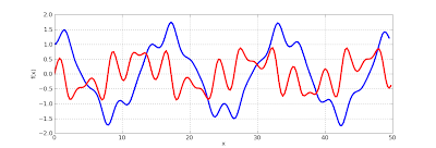
The Mathieu function and its derivative can be plotted as follows, showing complex, quasi-periodic behavior:
    >>> mp.dps = 5
    >>> f = odefun(lambda x,y: [y[1], cos(2*x)*y[0]], 0, [1, 0])
    >>> plot([lambda x: f(x)[0], lambda x: f(x)[1]], [0, 50])

Infinite sums & products
The sumsh and sumrich functions for summation of infinite series have been replaced by a single function nsum which is much more user friendly. nsum automatically chooses the appropriate extrapolation algorithm and figures out how many terms are needed to converge to the target precision. For most sums, nsum will quickly give the correct result automatically. The user can still tweak the settings to improve speed (in bad cases, tweaking is still necessary to obtain a correct result).
Here are two slowly convergent sums. Running with "verbose=True" would show that nsum automatically uses Richardson extrapolation for the first and Shanks transformation for the second:
    >>> mp.dps = 30
    >>> print nsum(lambda k: 1 / k**4, [1,inf])
    1.08232323371113819151600369654
    >>> print nsum(lambda k: (-1)**k / (k*log(k)), [2,inf])
    0.526412246533310410930696501411
For sums that don't alternate or converge either at a geometric or polynomial rate, one must fall back to Euler-Maclaurin summation (this algorithm is not used by default, because it leads to unreasonable slowness in some cases):
    >>> print nsum(lambda k: 1/(k**2.5*log(k)), [2,inf], method='euler-maclaurin')
    0.370060942712738560920262150476
A fun fact is that nsum can sum (some) divergent Taylor series. The generating function of the Fibonacci numbers may be used to demonstrate:
    >>> x = mpf(10)
    >>> print nsum(lambda k: fib(k) * x**k, [0, inf])
    -0.0917431192660550458715596330275
    >>> print x/(1-x-x**2)
    -0.0917431192660550458715596330275
Also new is a function nprod which computes infinite products in exactly the same way as nsum. The limit function has also been updated to use the same adaptive algorithm as nsum. Ergo, two silly ways to compute π:
    # Wallis' product
    >>> print 2*nprod(lambda k: (4*k**2)/(4*k**2-1), [1, inf])
    3.14159265358979323846264338328

    # Stirling's formula
    >>> print limit(lambda n: fac(n) / (sqrt(n)*(n/e)**n), inf)**2 / 2
    3.14159265358979323846264338328
Calculus
diff can now be used to compute high-order derivatives:
    >>> mp.dps = 15
    >>> print diff(lambda x: 1/(1+sqrt(x)), 2.5, 100)
    6.473750316944e+114
As a consequence, one can now compute Taylor series of arbitrary functions:
    >>> for c in taylor(gamma, 1.0, 10):
    ...     print c
    ...
    1.0
    -0.577215664901533
    0.989055995327973
    -0.907479076080886
    0.9817280868344
    -0.981995068903145
    0.993149114621276
    -0.996001760442431
    0.998105693783129
    -0.999025267621955
    0.999515656072777
There is also support for computing and evaluating Fourier series on arbitrary intervals. The Fourier coefficients are simply calculated using numerical integration, so this is not a fundamentally new feature; just an added convenience (I always find the scaling and translation factors in Fourier series a big pain).
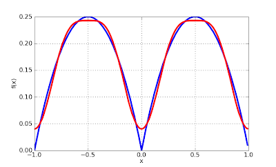
Let's plot the Fourier approximation of degree 2 for the periodic extension of x*(1-x) on [0, 1]. The sine coefficients vanish because the function's symmetry:
    >>> def f(x):
    ...     x = x % 1
    ...     return x*(1-x)
    ...
    >>> c, s = fourier(f, [0, 1], 2)
    >>> nprint(c)
    [0.166667, -0.101321, -2.53303e-2]
    >>> nprint(s)
    [0.0, 0.0, 0.0]
    >>> plot([f, lambda x: fourierval((c,s), [0,1], x)], [-1, 1])

Multidimensional rootfinding
The last new feature I'll demonstrate is multidimensional rootfinding, which has been implemented by Vinzent Steinberg (who also wrote the 1D rootfinding code in mpmath).
A useful application of multidimensional rootfinding is nonlinear interpolation. Vinzent suggested the following example: let h(t) = 220 / (1 + b*exp(-a*t)) describe the growth of a plant and let h(5) = 20.4 and h(10) = 92.9. To determine the parameters a and b based on this data, we do:
    >>> mp.dps = 15
    >>> h1 = lambda a, b: 220 / (1 + b*exp(-a*5)) - 20.4
    >>> h2 = lambda a, b: 220 / (1 + b*exp(-a*10)) - 92.9
    >>> findroot([h1, h2], (0, 1))
    matrix(
    [['0.393465986130316'],
     ['69.9730657971833']])
I'll finish with a high-precision example. Consider the ellipse defined by x2/2 + y2/3 = 2 and the hyperbola xy = 1. They intersect at four points, of which two are located in the first quadrant (the other two are given by mirror symmetry).
    >>> mp.dps = 30
    >>> f1 = lambda x,y: x**2/2+y**2/3-2
    >>> f2 = lambda x,y: x*y-1
    >>> x1, y1 = findroot([f1, f2], [2,1])
    >>> x2, y2 = findroot([f1, f2], [1,2])
    >>> print x1, y1
    1.95595037215941491574250931301 0.511260415516563762762967836065
    >>> print x2, y2
    0.417442381232962842628208975047 2.3955401869987133587345757307
We can now reliably find exact expressions for the intersection points by passing the approximations to the PSLQ algorithm:
    >>> identify(x1), identify(y1)
    ('sqrt(((12+sqrt(120))/6))', 'sqrt(((12-sqrt(120))/4))')
    >>> identify(x2), identify(y2)
    ('sqrt(((12-sqrt(120))/6))', 'sqrt(((12+sqrt(120))/4))')
That's it for now! Bug reports are as usual welcome on the issue tracker.
