Friday, February 12, 2010

Numerical multidimensional infinite series

Another new feature in mpmath: support for multidimensional series in nsum. Some very simple examples (finite and infinite summations can be combined in any desired order):

>>> nsum(lambda i,j: 2**(-i-j), [0,inf], [0,inf])
4.0
>>> nsum(lambda i,j,k: 2**(-i-j-k), [0,inf], [0,inf], [0,inf])
8.0
>>> nsum(lambda i,j,k,l: i/2**j*(i+l)/2**k, [1,2], [0,inf], [1,inf], [2,3])
50.0
>>> nsum((lambda i,j,k,l: 1/(2**(i**2+j**2+k**2+l**2))), *([[-inf,inf]]*4))
20.5423960756379
>>> jtheta(3,0,0.5)**4
20.5423960756379

One could of course also make nested calls to nsum, but having a direct syntax is much more convenient. Nested evaluation is also usually inefficient for convergence acceleration, so this is not what nsum does internally. Instead, it combines all the infinite summations to a single summation over growing hypercubes. The distinction is very important for conditionally convergent series.

For example, nsum can now directly evaluate the Madelung constant in three dimensions (ignore=True is to ignore the singular term at the origin):

>>> nsum(lambda i,j,k: (-1)**(i+j+k)/(i**2+j**2+k**2)**0.5,
... [-inf,inf], [-inf,inf], [-inf,inf], ignore=True)
-1.74756459463318


While this evaluation takes several seconds, it is somewhat remarkable that a precise value can be obtained at all. A better way to compute the Madelung constant is using the following rapidly convergent 2D series:

>>> f = lambda i,j: -12*pi*sech(0.5*pi*sqrt((2*i+1)**2+(2*j+1)**2))**2
>>> nsum(f, [0,inf], [0,inf])
-1.74756459463318
>>> mp.dps = 100
>>> nsum(f, [0,inf], [0,inf])
-1.74756459463318219063621203554439740348516143662474175815282535076504062353276
117989075836269460789


Another nice application is to evaluate Eisenstein series directly from the definition:

>>> tau = 1j
>>> q = qfrom(tau=tau)
>>> nsum(lambda m,n: (m+n*tau)**(-4), [-inf,inf], [-inf,inf], ignore=True)
(3.1512120021539 + 0.0j)
>>> 0.5*sum(jtheta(n,0,q)**8 for n in [2,3,4])*(2*zeta(4))
(3.1512120021539 + 0.0j)

Thursday, February 11, 2010

A new gamma function implementation

The gamma function is probably the most important nonelementary special function. The gamma function or ratios of gamma functions appear in everything from the functional equation of the Riemann zeta function to the normalization factors of hypergeometric functions. Even expressions that are usually rational functions (such as binomial coefficients) are often most conveniently expressed (or in software, implemented) in terms of the gamma function since this automatically provides correct asymptotics and extension to noninteger parameters. Needless to say, a well-implemented gamma function is fundamental for a special functions library.

The gamma function implementation used in mpmath until now is one of the oldest parts of the code (I wrote it around three years ago), and although it has done its job, it has some flaws. It mainly uses Spouge's approximation, which is fairly efficient but nonoptimal for asymptotically large arguments. The implementation also has some subtle precision issues.

The new gamma function added in this commit is the result of over a year of intermittent work. I did most of the work during last summer but didn't have time to finish it until recently. The improvements are essentially the following:

  • Removal of various overheads

  • Special-casing half-integers

  • Using Taylor series for small real arguments

  • Using Stirling's series for complex and/or large arguments

  • Optimizing for computing loggamma

  • Handling values near poles and near the real axis extremely carefully


The difference in performance is quite dramatic. The smallest speedup occurs for small complex arguments, but it turns out that even there, the Stirling series is faster than Spouge's approximation (at least with the removal of overheads in the new implementation) despite the need to perform argument transformations. For real arguments, and large complex arguments, the new implementation is consistently faster by a large factor, especially for loggamma.

I'll show some benchmarks. The times are in milliseconds; the first value in each cell is the time for the old implementation and the second is the time for the new one, followed by the speedup. The results are on my laptop, with gmpy (I'll try with Sage later):

Firstly, results for gamma(z):

zdps=15dps=50dps=250dps=1000
3.00.0086
0.0077
(1.13x)
0.0089
0.0076
(1.16x)
0.0087
0.0075
(1.16x)
0.0085
0.0077
(1.12x)
5.270.1200
0.0342
(3.51x)
0.2513
0.0545
(4.61x)
2.5964
0.4220
(6.15x)
80.7089
11.3011
(7.14x)
2.50.1255
0.0158
(7.94x)
0.2398
0.0138
(17.41x)
2.5519
0.0144
(177.72x)
79.0651
0.0149
(5319.87x)
-3.70.2518
0.0457
(5.51x)
0.4006
0.0615
(6.52x)
3.1073
0.4283
(7.26x)
87.4200
11.3981
(7.67x)
(-3.0+4.0j)0.6205
0.3942
(1.57x)
1.0095
0.6093
(1.66x)
9.0896
5.9099
(1.54x)
253.9219
191.3358
(1.33x)
(3.25-4.125j)0.3548
0.2864
(1.24x)
0.7456
0.4791
(1.56x)
8.6651
5.6367
(1.54x)
252.7598
189.2187
(1.34x)
(15.0+20.0j)0.3980
0.1973
(2.02x)
0.7526
0.4496
(1.67x)
8.6583
5.4604
(1.59x)
250.8646
188.5849
(1.33x)
52.10.1661
0.0586
(2.83x)
0.3050
0.0894
(3.41x)
2.9862
0.5685
(5.25x)
84.8334
12.4169
(6.83x)
123.250.1643
0.0638
(2.57x)
0.3071
0.0963
(3.19x)
2.8908
0.9194
(3.14x)
83.8168
14.6588
(5.72x)
-200.70.3011
0.1485
(2.03x)
0.4897
0.1914
(2.56x)
3.5145
1.1359
(3.09x)
89.8617
17.5500
(5.12x)
(100.25+100.0j)0.4238
0.1857
(2.28x)
0.7641
0.2757
(2.77x)
8.6807
3.1403
(2.76x)
249.6731
171.4369
(1.46x)
12345678.90.3032
0.0701
(4.32x)
0.4382
0.0857
(5.11x)
3.4078
0.3257
(10.46x)
88.4082
5.2828
(16.74x)
(0.0+12345678.9j)0.7814
0.1409
(5.54x)
1.1671
0.1802
(6.48x)
10.3985
0.6169
(16.86x)
265.6192
8.3569
(31.78x)
1.0e+200.8833
0.0798
(11.06x)
1.3019
0.0899
(14.48x)
6.4010
0.2939
(21.78x)
107.0924
3.5141
(30.47x)
(0.0+1.0e+20j)3.5025
0.1515
(23.11x)
3.6163
0.1834
(19.72x)
19.5676
0.5308
(36.86x)
322.9033
6.2148
(51.96x)


Secondly, results for loggamma(z):

zdps=15dps=50dps=250dps=1000
3.00.0700
0.0115
(6.07x)
0.0677
0.0116
(5.84x)
0.0683
0.0119
(5.73x)
0.0683
0.0121
(5.65x)
5.270.2207
0.0564
(3.91x)
0.3548
0.0796
(4.45x)
2.8925
0.5221
(5.54x)
88.3556
12.6452
(6.99x)
2.50.2210
0.0319
(6.93x)
0.3565
0.0374
(9.53x)
2.8595
0.1011
(28.28x)
81.8333
1.3546
(60.41x)
-3.70.4392
0.0782
(5.62x)
0.6418
0.0987
(6.50x)
3.5767
0.5429
(6.59x)
88.8484
12.7363
(6.98x)
(-3.0+4.0j)1.1235
0.4942
(2.27x)
1.5685
0.7224
(2.17x)
10.0879
6.0459
(1.67x)
267.2893
198.7613
(1.34x)
(3.25-4.125j)0.8789
0.2704
(3.25x)
1.2326
0.4752
(2.59x)
9.7501
5.4572
(1.79x)
264.7649
190.4007
(1.39x)
(15.0+20.0j)0.8983
0.1248
(7.20x)
1.2923
0.4221
(3.06x)
9.7917
5.2766
(1.86x)
265.2711
187.9775
(1.41x)
52.10.2604
0.0812
(3.21x)
0.4186
0.1140
(3.67x)
3.2493
0.6890
(4.72x)
87.0111
13.9280
(6.25x)
123.250.2629
0.0478
(5.50x)
0.4227
0.0692
(6.11x)
3.1110
1.0216
(3.05x)
85.9028
15.9917
(5.37x)
-200.70.5439
0.1631
(3.34x)
0.7465
0.2221
(3.36x)
3.9305
1.2537
(3.14x)
92.5380
18.8309
(4.91x)
(100.25+100.0j)0.9103
0.1179
(7.72x)
1.3332
0.1849
(7.21x)
10.1655
3.1083
(3.27x)
266.3565
170.3099
(1.56x)
12345678.90.4026
0.0491
(8.21x)
0.5439
0.0525
(10.36x)
3.7183
0.2051
(18.13x)
89.9402
4.0044
(22.46x)
(0.0+12345678.9j)1.2628
0.0765
(16.52x)
1.7085
0.0858
(19.91x)
11.5023
0.2749
(41.84x)
275.6174
4.4548
(61.87x)
1.0e+200.9820
0.0495
(19.84x)
1.3882
0.0540
(25.72x)
6.6983
0.1481
(45.21x)
110.1757
2.1954
(50.19x)
(0.0+1.0e+20j)4.0385
0.0788
(51.24x)
4.3758
0.0833
(52.54x)
20.9478
0.1936
(108.20x)
335.9407
2.3911
(140.50x)


All times are from a warm cache. The new implementation has slightly longer precomputation time (for the Taylor series coefficients) at high precision, and the Taylor series therefore isn't used above a certain precision (around 1000 digits) despite being much faster on subsequent calls. I will probably add some user-visible function for controlling this.

Finally, several optimizations are possible still. The most important would be to do the implementation in Cython. (Improving the underlying elementary functions will also speed up the gamma function.) Potential algorithmic improvements include faster handling of near-integers (using Taylor series with a reduced number of terms), avoiding the reflection formula for complex arguments in the left half-plane but not too close to the negative half-axis, and performing the argument transformations with a reduced number of multiplications. But I doubt I will have time (or interest -- the present code was demanding enough to finish) to work of any of these things, at least any time soon.

The speedups naturally also affect performance of many other functions, e.g. hypergeometric functions; I might post some benchmarks of that later.

Friday, February 5, 2010

Mpmath 0.14 released

I've just released version 0.14 of mpmath! Some highlights in this release have been covered in previous development updates on this blog:

  • mpmath in Sage to become 3x faster -- a Cython extension module will be added to Sage that greatly speeds up mpmath (the Sage patch is currently being reviewed; if all goes to plan, the patch will be accepted soon and the mpmath version in Sage will be updated to 0.14 at the same time).

  • Zeta evaluation with the Riemann-Siegel expansion -- Juan Arias de Reyna contributed code for very efficient and robust evaluation of the Riemann zeta function for arguments with large imaginary part.

  • Various features discussed in this update: 3D surface plotting (wrapping matplotlib, matrix calculus (transcendental functions of a matrix argument), Borel summation of divergent hypergeometric series, and options for whether to use Mathematica's conventions for hypergeometric functions have been added.

  • Improved accuracy for hypergeometric functions with large parameters, and analytic continuation implemented for 3F2, 4F3, and higher hypergeometric functions.

  • Support for using Python floats/complexes for faster low-precision math. This is very handy for plotting, multidimensional integration, and other things requiring many function evaluations.

There are many other changes as well. See the CHANGES file and the list of commits for more details. Thanks to Juan Arias de Reyna, Vinzent Steinberg, Jorn Baayen and Chris Smith who contributed patches, and various people who tested and submitted bug reports (thanks also to anyone else I forgot to mention).

I'm sorry that it took several months to finish this release! This was partly due to large internal reorganizations done in order to support floats and the Cython backend in Sage. I've also had to take some time off to focus on my studies and other things.

An example: spherical harmonics


Here I will demonstrate three new features with a single example: 3D plotting, one of the newly added special functions (spherical harmonics), and low-precision evaluation with the fp context. Of course, everything here can be done in arbitrary precision with mp as well; fp is just faster for plotting.

The following code visualizes spherical harmonics using a 3D polar plot. I've chosen to visualize the real part; the code is easily edited to show the absolute value (for example) instead.

from mpmath import fp

def Y(m,n):
def g(theta,phi):
R = fp.re(fp.spherharm(m,n,theta,phi))**2
x = R*fp.cos(phi)*fp.sin(theta)
y = R*fp.sin(phi)*fp.sin(theta)
z = R*fp.cos(theta)
return [x,y,z]
return g

fp.splot(Y(0,0), [0,fp.pi], [0,2*fp.pi])

The first few spherical harmonics are thus:
Y(0,0)
Y(1,0)
Y(1,1)
Y(2,0)
Y(2,1)
Y(2,2)
Y(3,0)
Y(3,1)
Y(3,2)
Y(3,3)


Some numerical examples


A selection of evaluations that were not implemented, failed, gave inaccurate results or were extremely slow in previous versions of mpmath:


>>> from mpmath import *
>>> mp.dps = 25; mp.pretty = True

# reflection formula for Barnes G-function
>>> barnesg(-100000+10000j)
(-7.332534002219787256775675e+22857579769 +
1.304469872717249495403882e+22857579770j)

# Riemann zeta function, large height
>>> zeta(0.5+100000000j)
(-3.362839487530727943146807 + 1.407234559646447885979583j)

# Accurate evaluation of large-degree Bernoulli polynomial
>>> bernpoly(1000,100)
4.360903799140670486890619e+1996

# Computation of Euler numbers
>>> eulernum(20)
370371188237525.0
>>> eulernum(50, exact=True)
-6053285248188621896314383785111649088103498225146815121L
>>> eulernum(2000000000000000000)
3.19651108713502662532039e+35341231273461153426

# Accurate evaluation of hypergeometric functions with large parameters
>>> hyp2f1(1000,50,25,-1)
-2.886992344761576738138864e-274
>>> legenp(0.5, 300, 0.25)
-1.717508549497252387888262e+578
>>> besseli(2, 10, derivative=100)
821.2386210064833486609255

# Evaluation of 4F3 and 4F2
>>> hyper([1,2.125,3.25,4.5], [5.25,6.5,7], 1+2j)
(1.006737556189825231039221 + 0.3058770612264986390003873j)
>>> hyper([1,2.125,3.25,4.5], [5.25,6.5], 1+2j)
(0.3220085070641791195103201 + 0.5251231752161637627314328j)

# Matrix functions
>>> A = matrix([[2,3,1+j],[1,0,-1],[2,1,5]])
>>> mnorm(A - logm(expm(A)))
9.540212722670391941827867e-25
>>> mnorm(A - expm(logm(A)))
4.375286550134565812513542e-26
>>> nprint(expm(2*A))
[ (-2855.4 + 10733.0j) (-1871.95 + 8597.9j) (-7721.42 + 12906.7j)]
[(-3910.68 - 1749.82j) (-3152.69 - 1272.11j) (-4460.18 - 3558.54j)]
[ (17039.0 + 22621.8j) (14320.3 + 17405.9j) (13587.7 + 35087.8j)]
>>> nprint(expm(A)**2)
[ (-2855.4 + 10733.0j) (-1871.95 + 8597.9j) (-7721.42 + 12906.7j)]
[(-3910.68 - 1749.82j) (-3152.69 - 1272.11j) (-4460.18 - 3558.54j)]
[ (17039.0 + 22621.8j) (14320.3 + 17405.9j) (13587.7 + 35087.8j)]
>>> nprint(chop(sqrtm(A)*sqrtm(A)))
[2.0 3.0 (1.0 + 1.0j)]
[1.0 0.0 -1.0]
[2.0 1.0 5.0]

# A convenience function for precise evaluation of exp(j*pi*x)
>>> expjpi(36); exp(j*pi*36)
(1.0 + 0.0j)
(1.0 + 4.702307256907087875509661e-25j)

# Some fp functions have specialized implementations
# for improved speed and accuracy
>>> fp.erfc(5); float(mp.erfc(5))
1.5374597944280347e-12
1.5374597944280349e-12
>>> fp.erf(5); float(mp.erf(5))
0.99999999999846256
0.99999999999846256
>>> fp.ei(-12-3j); complex(mp.ei(-12-3j))
(4.6085637890261843e-07-3.141592693919709j)
(4.6085637890261901e-07-3.141592693919709j)
>>> fp.zeta(-0.5); float(fp.zeta(-0.5)) # real-argument fp.zeta
-0.20788622497735468
-0.20788622497735468
>>> fp.ci(40); float(mp.ci(40))
0.019020007896208769
0.019020007896208765
>>> fp.gamma(4+5j); complex(mp.gamma(4+5j))
(0.14965532796078551+0.31460331072967695j)
(0.14965532796078521+0.31460331072967596j)


For more examples and images, see the posts linked at the top of this post!

Monday, February 1, 2010

mpmath in Sage to become 3x faster

I've blogged previously about the potential speedups attainable by rewriting core parts of mpmath in Cython (here and here), but all I had back then was some standalone classes and functions that couldn't easily be integrated. Well, I now finally have a fully working, fully integrated Cython implementation of the mpf and mpc types (plus related utility functions) -- and it successfully runs the entire mpmath test suite!

On my computer (Ubuntu 64 bit, AMD Athlon 64 3700+), running import mpmath; mpmath.runtests() in Sage takes this much time:

Before [mpmath (svn trunk) + Sage 4.3.1]: 62.75 seconds

After [mpmath (svn trunk with modifications) + Cython mpmath types + Sage 4.3.1 + a Sage performance patch by Robert Bradshaw]: 19.87 seconds

I have essentially only implemented arithmetic operations and conversions, so core transcendental functions (as well as square roots and powers) still fall back to the Python code, and they account for the majority of the running time. According to cProfile, about 20% of the total time is spent in exp() and gamma() alone. Hypergeometric series evaluation is also still done in Python. Replacing these functions with Cython versions should give a significant boost, and will be very easy to do in the future (in terms of code infrastructure). So realistically, the running time for the unit tests can be cut much further, probably in half.

The code isn't public yet. I will soon commit the changes to the mpmath svn repository and create a patch for Sage with the Cython extensions. The code just needs a little more cleanup, and there are no doubt a couple of subtle issues (such as corner-case memory leaks) that need fixing... but essentially, it's working, and the tests pass, so I expect it to be releasable quite soon.

Update: after adding just a little more Cythonized wrapper code, the time is now down to 17.64 seconds. I have still not touched exp, log, cos, sin, gamma, or any other core transcendental functions. Expect further improvements.

Update 2 (2010-02-03): preliminary version of the Cython code here

Wednesday, January 27, 2010

Using Sage numbers in mpmath

I've written a very basic mpmath context for computing "natively" with Sage's real and complex numbers. It can be tried out by upgrading mpmath in Sage to the svn trunk, applying this patch this patch to fix the helper code in Sage, and then importing this file.

Some examples:


----------------------------------------------------------------------
| Sage Version 4.3.1, Release Date: 2010-01-20 |
| Type notebook() for the GUI, and license() for information. |
----------------------------------------------------------------------
sage: from mpsage import SageContext
sage: from mpmath import mp, timing
sage: mp.prec = 150
sage: sc = SageContext(150)
sage:
sage: print sc.quad(lambda t: sc.exp(-t**2), [0,sc.inf])
0.88622692545275801364908374167057259139877471
sage: print mp.quad(lambda t: mp.exp(-t**2), [0,mp.inf])
0.88622692545275801364908374167057259139877473
sage: timing(sc.quad, lambda t: sc.exp(-t**2), [0,sc.inf])
0.40903496742248535
sage: timing(mp.quad, lambda t: mp.exp(-t**2), [0,mp.inf])
0.43610286712646484
sage:
sage: print sc.zeta(4+5*I)
0.95121830700949569861514024576822624312072806 + 0.024932824507357722259855155244740571939365897*I
sage: print mp.zeta(4+5*I, method='euler-maclaurin')
(0.95121830700949569861514024576822624312072806 + 0.024932824507357722259855155244740571939365897j)
sage: timing(sc.zeta, 4+5*I)
0.015111517906188966
sage: timing(mp.zeta, 4+5*I, method='euler-maclaurin')
0.028736209869384764
sage:
sage: print sc.zeta(1+100000000*I)
1.8349308953278466065175598876062914152382527 + 1.0691847904236128969174476736978194200591565*I
sage: print mp.zeta(1+100000000*I)
(1.8349308953278466065175598876062914152563156 + 1.069184790423612896917447673697819420203942j)
sage: timing(sc.zeta, 1+100000000*I)
1.0952680110931396
sage: timing(mp.zeta, 1+100000000*I)
2.0537140369415283


Unfortunately, there are some issues (besides the fact that some methods are missing, so not everything works yet).

This context doesn't provide variable precision, so the user has to manually allocate sufficient extra precision to compensate for rounding errors.

I first tried to do it, but variable precision is very inconvenient to implement using Sage's way of managing precision. There is no direct way to perform operations with a given target precision (independent of the inputs), and the second best option (which is to perform coercions to the target precision everywhere) is very slow, besides losing accuracy. The only way to implement variable precision in a reasonable way is to bypass Sage's RealNumber and ComplexNumber (at least their public interfaces) and wrap MPFR directly using a precision model similar to what MPFR and mpmath uses, where the precision of the result is always specified and independent of the inputs.

Secondly, there is not that much of a speedup (in the examples above, the speedup is at most about 2x). This is mainly due to the fact that the context uses wrapper classes for RealNumber and ComplexNumber, with all interface and conversion code written in Python. So the overhead is about the same as for the corresponding code in vanilla mpmath (where it accounts for about 50% of the total overhead). The reason RealNumber and ComplexNumber can't be used directly, even in a fixed-precision setting, is that mpmath in many places multiplies numbers by floats (usually exact float literals like 0.5), and Sage always coerces to the number with less precision. This could presumably be fixed by replacing all float and complex constants in mpmath, but I'm not in the mood to do that right now.

There should be a significant performance benefit if direct-from-Cython classes and conversion methods were used. It's also very important to optimize certain core functions; for example, quadrature would benefit greatly from a fast fdot implementation.

All things considered, I'm probably not going to continue much more down this particular path. It's better to write a fully compatible Cython context with classes designed directly for mpmath. Trying to wrap Sage's numbers did however help identify a few problems with the existing interfaces, so I might extend the work on this context a little more just to find more such issues.

Tuesday, January 19, 2010

Zeta evaluation with the Riemann-Siegel expansion

I'm very grateful to Juan Arias de Reyna who has contributed a module implementing zeta function evaluation using the Riemann-Siegel formula in mpmath. This finally permits rapid evaluation of the Riemann zeta function for arguments with large imaginary part.

To follow tradition on this blog, pictorial proof shall be given. Here is a plot of a segment of the critical line, ζ(1/2+ti) with t between 1010+50 and 1010+55:

A complex plot of showing the critical strip, t ranging between 108+40 and 108+45 (note: the y scale is reversed):


Juan Arias de Reyna, who is a professor of mathematics at the University of Seville, has done a thorough job with this code. He has even proved rigorous error bounds for his algorithm (subject to assumptions that the underlying functions in mpmath being well-implemented). The news is that the bounds -- documented in an as-yet unpublished paper -- are valid off the critical line. The code also computes derivatives (up to 4th derivatives), although not as rigorously but still very robustly.

I integrated the code (and added a few optimizations) during the last few days. The zeta function in mpmath now automatically switches between Borwein's algorithm (close to the real line), Euler-Maclaurin summation, and the Riemann-Siegel expansion.

Some example values and timings on my laptop, computing ζ(1/2+10ni) for n up to 12:

>>> from timeit import default_timer as clock
>>> mp.dps = 25
>>>
>>> for n in range(13):
... t1 = clock(); y = zeta(0.5 + 10**n*j); t2 = clock()
... print n, y, round(t2-t1,3)
...
0 (0.1439364270771890603243897 - 0.7220997435316730891261751j) 0.02
1 (1.544895220296752766921496 - 0.1153364652712733754365914j) 0.003
2 (2.692619885681324090476096 - 0.02038602960259816177072685j) 0.042
3 (0.3563343671943960550744025 + 0.9319978312329936651150604j) 0.073
4 (-0.3393738026388344575674711 - 0.03709150597320603147434421j) 0.434
5 (1.073032014857753132114076 + 5.780848544363503984261041j) 0.167
6 (0.07608906973822710000556456 + 2.805102101019298955393837j) 0.146
7 (11.45804061057709254500227 - 8.643437226836021723818215j) 0.181
8 (-3.362839487530727943146807 + 1.407234559646447885979583j) 0.336
9 (-2.761748029838060942376813 - 1.677512240989459839213205j) 0.877
10 (0.3568002308560733825395879 + 0.286505849095836103292093j) 2.695
11 (0.6436639255801185727194357 + 0.1168615914616853418448829j) 8.583
12 (2.877961809278403355251079 - 3.206771071318398923493412j) 26.934


Similar results off the critical line:

>>> for n in range(13):
... t1 = clock(); y = zeta(1.0 + 10**n*j); t2 = clock()
... print n, y, round(t2-t1,3)
...
0 (0.5821580597520036481994632 - 0.9268485643308070765364243j) 0.021
1 (1.390287313237401426796005 - 0.109785153066302056909746j) 0.004
2 (1.632833506686711866610705 - 0.06813120384181249010120548j) 0.043
3 (0.9409368682927533108010138 + 0.04522665207209509908865644j) 0.083
4 (0.4973279229716308441790286 - 0.5878238243194009766923214j) 0.598
5 (1.618122122846936796567759 + 1.070441041470623686626035j) 0.233
6 (0.9473872625104789104802422 + 0.5942199931209183283333071j) 0.195
7 (2.859846483332530337008882 + 0.491808047480981808903986j) 0.409
8 (1.83493089532784660651756 + 1.069184790423612896917448j) 0.455
9 (0.9038018561650776977609945 - 1.189857828822373901473908j) 1.393
10 (0.5418173564211820524034624 + 0.635303581895880322679247j) 3.824
11 (0.5365466615361310937110304 - 0.1234443975100346650640542j) 12.031
12 (0.8225630719679733497367277 - 0.4484762282040223492401122j) 38.061


The implementation also supports use of the fp context. Double precision unavoidably becomes insufficient as the imaginary part approaches 1015, but it has the advantage of speed in the range where it works:

>>> for n in range(13):
... t1 = clock(); y = fp.zeta(0.5 + 10**n*1j); t2 = clock()
... print n, y, round(t2-t1,3)
...
0 (0.143936427077-0.722099743532j) 0.007
1 (1.5448952203-0.115336465271j) 0.001
2 (2.69261988568-0.0203860296026j) 0.003
3 (0.356334367195+0.931997831233j) 0.004
4 (-0.339373802616-0.0370915059691j) 0.123
5 (1.07303201485+5.78084854433j) 0.005
6 (0.076089072636+2.80510210471j) 0.006
7 (11.4580404601-8.64343725721j) 0.006
8 (-3.36283920435+1.40723433071j) 0.011
9 (-2.76174796643-1.67750591108j) 0.028
10 (0.356829034142+0.286525774475j) 0.083
11 (0.64314751322+0.116713738713j) 0.256
12 (2.8689206645-3.21135962379j) 0.808


We have done some comparison with Mathematica, and the mpmath version appears to be about as fast (a bit faster or a bit slower, sometimes substantially faster, depending on circumstance). The most expensive part of the computation occurs in a simple internal function that adds lots of n−s terms. I think for Sage, it will be very easy to switch to a Cython version of this function which should improve speed by a large factor.

But most importantly, Mathematica's Zeta[] is notoriously buggy for large imaginary arguments. As a first example, here Mathematica 7.0 computes two entirely different values at different precisions:

In[3]:= N[Zeta[1/4+10^12 I], 15]
Out[3]= -0.0125397 + 0.0139723 I
In[4]:= N[Zeta[1/4+10^12 I], 30]
Out[4]= 358.066828240154490750947835567 - 580.623633400912069466146291259 I


With mpmath:

>>> mp.dps = 15; zeta(0.25+1e12j)
(358.066828240154 - 580.623633400912j)
>>> mp.dps = 30; zeta(0.25+1e12j)
(358.066828240154490750947835567 - 580.623633400912069466146291259j)


As a second example, if Mathematica is asked for derivatives, it's more likely than not to return complete nonsense, and even increasing the precision doesn't help:

In[2]:= N[Zeta'[1/2+10^6 I], 15]

883 883
Out[2]= 2.48728166483172 10 - 7.66644043045624 10 I

In[3]:= N[Zeta'[1/2+10^6 I], 25]

940 940
Out[3]= 1.586685034587255948191759 10 + 2.158475809806136995106119 10 I

In[4]:= N[Zeta'[1/2+10^6 I], 30]

1022
Out[4]= -1.071044014417407205715473623855 10 -

1021
> 2.73478073192015960107298455871 10 I


For contrast, mpmath computes derivatives perfectly:

>>> mp.dps = 15; zeta(0.5+1e6j, derivative=1)
(11.6368040660025 - 17.127254072213j)
>>> mp.dps = 25; zeta(0.5+1e6j, derivative=1)
(11.63680406600252145919591 - 17.12725407221299600357895j)
>>> mp.dps = 30; zeta(0.5+1e6j, derivative=1)
(11.6368040660025214591959071246 - 17.1272540722129960035789468265j)
>>> diff(zeta, 0.5+1e6j) # Numerical verification
(11.6368040660025214591959071246 - 17.1272540722129960035789468265j)


That's all for now. I'm back in school again, so maybe I won't have as much time for programming in the near future. But my schedule is flexible, so we'll see. A new release of mpmath shouldn't be far away.

Update: I should point out that the bugs in Mathematica's Zeta[] only seem to occur in recent versions. Mathematica 5 and older versions do not seem to have these problems.

Wednesday, January 13, 2010

YAMDU (yet another mpmath development update)

At the moment, I'm able to get quite a bit of work done on mpmath. This includes general code cleanup, gardening the issue tracker, and finishing features that were works-in-progress for a long while.

Today's topics are:

3D plotting
Matrix calculus
Borel summation of divergent hypergeometric series
Optional consistency with Mathematica
Internal reorganization

3D plotting


Jorn Baayen submitted a patch that adds 3D surface plotting (along with some other minor changes to the visualization module). Thanks a lot! I previously blogged about 3D plotting using matplotlib.

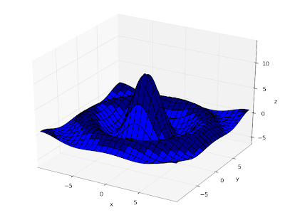
You can now easily produce plots of functions of the form z = f(x,y):

splot(lambda x, y: 10*sinc(hypot(x,y)), [-10,10], [-10,10])


You can just as easily plot more general parametric functions x,y,z = f(u,v). The following plots a Möbius strip:

def f(u,v):
d = (1+0.5*v*cos(0.5*u))
x = d*cos(u)
y = d*sin(u)
z = 0.5*v*sin(0.5*u)
return x,y,z

splot(f, [0,2*pi], [-1,1])
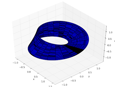


(I'm not sure why there are black spots in the image. This seems to be a matplotlib bug.)

Matrix calculus


It's now possible to compute exponentials, sines, cosines, square roots, logarithms, and complex powers (Az) of square matrices:


>>> mp.dps = 25; mp.pretty = True
>>> A = matrix([[2,3,1+j],[1,0,-1],[2,1,5]])
>>> nprint(expm(A))
[ (27.6034 + 41.2728j) (24.9924 + 31.1189j) (8.67256 + 68.271j)]
[(-15.0962 + 1.51713j) (-10.1713 + 1.30035j) (-28.7003 - 0.401789j)]
[ (125.368 + 37.7417j) (98.9812 + 26.9693j) (158.616 + 85.1593j)]
>>> nprint(logm(expm(A)))
[(2.0 - 5.35398e-26j) (3.0 + 6.9172e-26j) (1.0 + 1.0j)]
[(1.0 + 4.94422e-26j) (4.42102e-25 - 1.14411e-25j) (-1.0 - 1.95948e-27j)]
[(2.0 + 1.58966e-26j) (1.0 - 8.57028e-27j) (5.0 + 3.23653e-27j)]
>>> nprint(sqrtm(A)**2)
[(2.0 - 8.25839e-30j) (3.0 - 8.40399e-30j) (1.0 + 1.0j)]
[(1.0 + 4.63764e-30j) (4.84564e-30 - 3.27721e-31j) (-1.0 + 7.47261e-31j)]
[(2.0 - 4.31871e-30j) (1.0 + 1.78726e-31j) (5.0 + 2.54582e-29j)]
>>> nprint(powm(powm(A,1+j),1/(1+j)))
[(2.0 - 1.12995e-26j) (3.0 - 8.93158e-27j) (1.0 + 1.0j)]
[(1.0 - 1.54352e-26j) (9.23906e-27 - 1.67262e-26j) (-1.0 - 2.62243e-27j)]
[(2.0 + 9.97431e-27j) (1.0 + 1.56341e-26j) (5.0 - 1.79194e-26j)]


The code also works with the double precision fp context, which obviously is much faster for large matrices. When computing square roots and logarithms, most of the time is spent on matrix inversion, which can be accelerated by substituting in numpy:


>>> from mpmath import fp
>>> A = fp.randmatrix(20)
>>> B = fp.sqrtm(A)
>>> timing(fp.sqrtm, A)
3.6470590535948006
>>>
>>> import numpy
>>> fp.inverse = lambda A: fp.matrix(numpy.linalg.inv(A.tolist()))
>>>
>>> timing(fp.sqrtm, A)
1.0815329881311735
>>> C = fp.sqrtm(A)
>>>
>>> fp.mnorm(A-B**2)
3.5001514923930131e-14
>>> fp.mnorm(A-C**2)
2.6462503380426079e-14


It could be much faster still by doing everything in numpy. Probably in the future fp should be improved to seamlessly use numpy internally for all available matrix operations. Patches are welcome!

Borel summation of divergent hypergeometric series


The hypergeometric series of degree p > q+1 are divergent for |z| > 0. Nevertheless, they define asymptotic expansions for analytic functions which exist in the sense of Borel summation. Previously, mpmath knew only how to evaluate 2F0 (whose Borel sum has a closed form), but now it can evaluate the functions of higher degree as well.

To illustrate, the cosine integral Ci(z) has an asymptotic series representation in terms of 3F0:


This representation is efficient for very large values of |z|, where the argument of the hypergeometric series is small. But with z = 0.5, say, the series does not yield a single digit. With a value of z = 10 or so, the series only gives about 3 digits with an optimal truncation:

>>> z = 10.0
>>> for n in range(1,16):
... print sum(rf(0.5,k)*rf(1,k)*rf(1,k)*(-4/(z**2))**k/fac(k) for k in range(n))
...
1.0
0.98
0.9824
0.98168
0.9820832
0.98172032
0.9821993216
0.981327538688
0.9834198176768
0.977017443971072
1.00134646405284
0.888946391275078
1.50939479300832
-2.52351981825774
27.9653146429137


Of course, there are ways to compute the cosine integral using convergent series. But if we pretend that we only know about the asymptotic series, then the Borel regularization means that we can evaluate the function to high precision even for small z:

>>> mp.dps = 25; mp.pretty = True
>>> z = mpf(0.5)
>>> u = -4/z**2
>>> H1 = hyper([1,1,1.5],[],u)
>>> H2 = hyper([0.5,1,1],[],u)
>>>
>>> print log(z)-log(z**2)/2-cos(z)/z**2*H1+sin(z)/z*H2
-0.1777840788066129013358103
>>> print ci(z)
-0.1777840788066129013358103


The z = 10 series above, to high precision:

>>> hyper([0.5,1,1],[],-4/(10.0**2))
0.9819103501017016869905255
>>> mp.dps = 40
>>> hyper([0.5,1,1],[],-4/(10.0**2))
0.9819103501017016869905255431829554224704


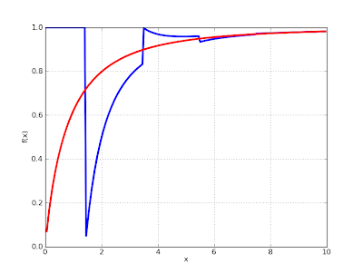
It's instructive to visualize the optimal truncations of an asymptotic series compared to the exact solution. Notice how, for an alternating series like this, the truncations alternate between over- and undershooting:

def optimal_asymp(z):
u = -4/(z**2)
term_prev = inf
s = 0.0
for k in range(30):
term = rf(0.5,k)*rf(1,k)*rf(1,k)*u**k/fac(k)
if abs(term) < abs(term_prev):
s += term
term_prev = term
else:
break
return s

def exact(z):
u = -4/(z**2)
return hyper([0.5,1,1],[],u)

mp.dps = 10
plot([optimal_asymp, exact], [0,10])


The catch with this feature? Computing the Borel regularization involves evaluating (nested) numerical integrals with a hypergeometric function in the integrand. Except for special parameters (where degree reductions happen internally -- the Ci series above happens to be such a case), it's not very fast.

Optional consistency with Mathematica


I often try to follow Mathematica's conventions regarding limits, special values and branch cuts of special functions. This simplifies testing (I can directly compare values with Mathematica), and usually Mathematica's conventions seem well-reasoned.

There are exceptions, however. One such exception concerns Mathematica's interpretation of 2F1(a,b,c,z) for b = c a negative integer. Mathematica interprets this as a polynomial, which doesn't make much sense since the denominator of the zero term is zero. It's not even consistent with how Mathematica evaluates this function for a symbolic variable:

In[3]:= Hypergeometric2F1[3,-2,-2,2]

Out[3]= 31

In[4]:= Hypergeometric2F1[3,b,b,2]

Out[4]= -1


Maybe there is a good reason for doing what Mathematica does, but it's at the very least not documented anywhere. I've now changed mpmath to instead interpret the two parameters as eliminating each other and giving a 1F0 function (which is what Mathematica does for a generic value). The Mathematica-compatible value can be recovered by explicitly disabling parameter elimination:

>>> mp.pretty = True
>>>
>>> hyp2f1(3,-2,-2,2)
-1.0
>>> hyp2f1(3,-2,-2,2,eliminate=False)
31.0


On a related note, I've fixed the Meijer G-function to switch between its z and 1/z forms automatically to follow Mathematica's definition of the function. This introduces discontinuities in the function for certain orders. The user can explicitly choose which form to use (so as to obtain a continuous function) with series=1 or series=2.

Internal reorganization


In a long overdue change, I've moved many of the modules in mpmath into subdirectories. The multiprecision library code is now located in mpmath/libmp; special functions are in mpmath/functions, calculus routines are in mpmath/calculus, and routines for matrices and linear algebra are in mpmath/matrices.

This shouldn't affect any documented interfaces, but it will break external code that directly uses mpmath internal functions. The mpmath interfaces in SymPy and Sage will need some editing for the next version update. The breakage should be straightforward to fix (mostly just a matter of changing imports).

Since the next version of mpmath is definitely going to break some code, I might use the opportunity to do some other cosmetic interface changes as well. Ideally, after the next version, the interface will be stable until and beyond mpmath 1.0 (whenever that happens). But the version number is still at 0.x for a reason -- no compatibility guarantees.
