Wednesday, January 27, 2010

Using Sage numbers in mpmath

I've written a very basic mpmath context for computing "natively" with Sage's real and complex numbers. It can be tried out by upgrading mpmath in Sage to the svn trunk, applying this patch this patch to fix the helper code in Sage, and then importing this file.

Some examples:


----------------------------------------------------------------------
| Sage Version 4.3.1, Release Date: 2010-01-20 |
| Type notebook() for the GUI, and license() for information. |
----------------------------------------------------------------------
sage: from mpsage import SageContext
sage: from mpmath import mp, timing
sage: mp.prec = 150
sage: sc = SageContext(150)
sage:
sage: print sc.quad(lambda t: sc.exp(-t**2), [0,sc.inf])
0.88622692545275801364908374167057259139877471
sage: print mp.quad(lambda t: mp.exp(-t**2), [0,mp.inf])
0.88622692545275801364908374167057259139877473
sage: timing(sc.quad, lambda t: sc.exp(-t**2), [0,sc.inf])
0.40903496742248535
sage: timing(mp.quad, lambda t: mp.exp(-t**2), [0,mp.inf])
0.43610286712646484
sage:
sage: print sc.zeta(4+5*I)
0.95121830700949569861514024576822624312072806 + 0.024932824507357722259855155244740571939365897*I
sage: print mp.zeta(4+5*I, method='euler-maclaurin')
(0.95121830700949569861514024576822624312072806 + 0.024932824507357722259855155244740571939365897j)
sage: timing(sc.zeta, 4+5*I)
0.015111517906188966
sage: timing(mp.zeta, 4+5*I, method='euler-maclaurin')
0.028736209869384764
sage:
sage: print sc.zeta(1+100000000*I)
1.8349308953278466065175598876062914152382527 + 1.0691847904236128969174476736978194200591565*I
sage: print mp.zeta(1+100000000*I)
(1.8349308953278466065175598876062914152563156 + 1.069184790423612896917447673697819420203942j)
sage: timing(sc.zeta, 1+100000000*I)
1.0952680110931396
sage: timing(mp.zeta, 1+100000000*I)
2.0537140369415283


Unfortunately, there are some issues (besides the fact that some methods are missing, so not everything works yet).

This context doesn't provide variable precision, so the user has to manually allocate sufficient extra precision to compensate for rounding errors.

I first tried to do it, but variable precision is very inconvenient to implement using Sage's way of managing precision. There is no direct way to perform operations with a given target precision (independent of the inputs), and the second best option (which is to perform coercions to the target precision everywhere) is very slow, besides losing accuracy. The only way to implement variable precision in a reasonable way is to bypass Sage's RealNumber and ComplexNumber (at least their public interfaces) and wrap MPFR directly using a precision model similar to what MPFR and mpmath uses, where the precision of the result is always specified and independent of the inputs.

Secondly, there is not that much of a speedup (in the examples above, the speedup is at most about 2x). This is mainly due to the fact that the context uses wrapper classes for RealNumber and ComplexNumber, with all interface and conversion code written in Python. So the overhead is about the same as for the corresponding code in vanilla mpmath (where it accounts for about 50% of the total overhead). The reason RealNumber and ComplexNumber can't be used directly, even in a fixed-precision setting, is that mpmath in many places multiplies numbers by floats (usually exact float literals like 0.5), and Sage always coerces to the number with less precision. This could presumably be fixed by replacing all float and complex constants in mpmath, but I'm not in the mood to do that right now.

There should be a significant performance benefit if direct-from-Cython classes and conversion methods were used. It's also very important to optimize certain core functions; for example, quadrature would benefit greatly from a fast fdot implementation.

All things considered, I'm probably not going to continue much more down this particular path. It's better to write a fully compatible Cython context with classes designed directly for mpmath. Trying to wrap Sage's numbers did however help identify a few problems with the existing interfaces, so I might extend the work on this context a little more just to find more such issues.

Tuesday, January 19, 2010

Zeta evaluation with the Riemann-Siegel expansion

I'm very grateful to Juan Arias de Reyna who has contributed a module implementing zeta function evaluation using the Riemann-Siegel formula in mpmath. This finally permits rapid evaluation of the Riemann zeta function for arguments with large imaginary part.

To follow tradition on this blog, pictorial proof shall be given. Here is a plot of a segment of the critical line, ζ(1/2+ti) with t between 1010+50 and 1010+55:

A complex plot of showing the critical strip, t ranging between 108+40 and 108+45 (note: the y scale is reversed):


Juan Arias de Reyna, who is a professor of mathematics at the University of Seville, has done a thorough job with this code. He has even proved rigorous error bounds for his algorithm (subject to assumptions that the underlying functions in mpmath being well-implemented). The news is that the bounds -- documented in an as-yet unpublished paper -- are valid off the critical line. The code also computes derivatives (up to 4th derivatives), although not as rigorously but still very robustly.

I integrated the code (and added a few optimizations) during the last few days. The zeta function in mpmath now automatically switches between Borwein's algorithm (close to the real line), Euler-Maclaurin summation, and the Riemann-Siegel expansion.

Some example values and timings on my laptop, computing ζ(1/2+10ni) for n up to 12:

>>> from timeit import default_timer as clock
>>> mp.dps = 25
>>>
>>> for n in range(13):
... t1 = clock(); y = zeta(0.5 + 10**n*j); t2 = clock()
... print n, y, round(t2-t1,3)
...
0 (0.1439364270771890603243897 - 0.7220997435316730891261751j) 0.02
1 (1.544895220296752766921496 - 0.1153364652712733754365914j) 0.003
2 (2.692619885681324090476096 - 0.02038602960259816177072685j) 0.042
3 (0.3563343671943960550744025 + 0.9319978312329936651150604j) 0.073
4 (-0.3393738026388344575674711 - 0.03709150597320603147434421j) 0.434
5 (1.073032014857753132114076 + 5.780848544363503984261041j) 0.167
6 (0.07608906973822710000556456 + 2.805102101019298955393837j) 0.146
7 (11.45804061057709254500227 - 8.643437226836021723818215j) 0.181
8 (-3.362839487530727943146807 + 1.407234559646447885979583j) 0.336
9 (-2.761748029838060942376813 - 1.677512240989459839213205j) 0.877
10 (0.3568002308560733825395879 + 0.286505849095836103292093j) 2.695
11 (0.6436639255801185727194357 + 0.1168615914616853418448829j) 8.583
12 (2.877961809278403355251079 - 3.206771071318398923493412j) 26.934


Similar results off the critical line:

>>> for n in range(13):
... t1 = clock(); y = zeta(1.0 + 10**n*j); t2 = clock()
... print n, y, round(t2-t1,3)
...
0 (0.5821580597520036481994632 - 0.9268485643308070765364243j) 0.021
1 (1.390287313237401426796005 - 0.109785153066302056909746j) 0.004
2 (1.632833506686711866610705 - 0.06813120384181249010120548j) 0.043
3 (0.9409368682927533108010138 + 0.04522665207209509908865644j) 0.083
4 (0.4973279229716308441790286 - 0.5878238243194009766923214j) 0.598
5 (1.618122122846936796567759 + 1.070441041470623686626035j) 0.233
6 (0.9473872625104789104802422 + 0.5942199931209183283333071j) 0.195
7 (2.859846483332530337008882 + 0.491808047480981808903986j) 0.409
8 (1.83493089532784660651756 + 1.069184790423612896917448j) 0.455
9 (0.9038018561650776977609945 - 1.189857828822373901473908j) 1.393
10 (0.5418173564211820524034624 + 0.635303581895880322679247j) 3.824
11 (0.5365466615361310937110304 - 0.1234443975100346650640542j) 12.031
12 (0.8225630719679733497367277 - 0.4484762282040223492401122j) 38.061


The implementation also supports use of the fp context. Double precision unavoidably becomes insufficient as the imaginary part approaches 1015, but it has the advantage of speed in the range where it works:

>>> for n in range(13):
... t1 = clock(); y = fp.zeta(0.5 + 10**n*1j); t2 = clock()
... print n, y, round(t2-t1,3)
...
0 (0.143936427077-0.722099743532j) 0.007
1 (1.5448952203-0.115336465271j) 0.001
2 (2.69261988568-0.0203860296026j) 0.003
3 (0.356334367195+0.931997831233j) 0.004
4 (-0.339373802616-0.0370915059691j) 0.123
5 (1.07303201485+5.78084854433j) 0.005
6 (0.076089072636+2.80510210471j) 0.006
7 (11.4580404601-8.64343725721j) 0.006
8 (-3.36283920435+1.40723433071j) 0.011
9 (-2.76174796643-1.67750591108j) 0.028
10 (0.356829034142+0.286525774475j) 0.083
11 (0.64314751322+0.116713738713j) 0.256
12 (2.8689206645-3.21135962379j) 0.808


We have done some comparison with Mathematica, and the mpmath version appears to be about as fast (a bit faster or a bit slower, sometimes substantially faster, depending on circumstance). The most expensive part of the computation occurs in a simple internal function that adds lots of ns terms. I think for Sage, it will be very easy to switch to a Cython version of this function which should improve speed by a large factor.

But most importantly, Mathematica's Zeta[] is notoriously buggy for large imaginary arguments. As a first example, here Mathematica 7.0 computes two entirely different values at different precisions:

In[3]:= N[Zeta[1/4+10^12 I], 15]
Out[3]= -0.0125397 + 0.0139723 I
In[4]:= N[Zeta[1/4+10^12 I], 30]
Out[4]= 358.066828240154490750947835567 - 580.623633400912069466146291259 I


With mpmath:

>>> mp.dps = 15; zeta(0.25+1e12j)
(358.066828240154 - 580.623633400912j)
>>> mp.dps = 30; zeta(0.25+1e12j)
(358.066828240154490750947835567 - 580.623633400912069466146291259j)


As a second example, if Mathematica is asked for derivatives, it's more likely than not to return complete nonsense, and even increasing the precision doesn't help:

In[2]:= N[Zeta'[1/2+10^6 I], 15]

883 883
Out[2]= 2.48728166483172 10 - 7.66644043045624 10 I

In[3]:= N[Zeta'[1/2+10^6 I], 25]

940 940
Out[3]= 1.586685034587255948191759 10 + 2.158475809806136995106119 10 I

In[4]:= N[Zeta'[1/2+10^6 I], 30]

1022
Out[4]= -1.071044014417407205715473623855 10 -

1021
> 2.73478073192015960107298455871 10 I


For contrast, mpmath computes derivatives perfectly:

>>> mp.dps = 15; zeta(0.5+1e6j, derivative=1)
(11.6368040660025 - 17.127254072213j)
>>> mp.dps = 25; zeta(0.5+1e6j, derivative=1)
(11.63680406600252145919591 - 17.12725407221299600357895j)
>>> mp.dps = 30; zeta(0.5+1e6j, derivative=1)
(11.6368040660025214591959071246 - 17.1272540722129960035789468265j)
>>> diff(zeta, 0.5+1e6j) # Numerical verification
(11.6368040660025214591959071246 - 17.1272540722129960035789468265j)


That's all for now. I'm back in school again, so maybe I won't have as much time for programming in the near future. But my schedule is flexible, so we'll see. A new release of mpmath shouldn't be far away.

Update: I should point out that the bugs in Mathematica's Zeta[] only seem to occur in recent versions. Mathematica 5 and older versions do not seem to have these problems.

Wednesday, January 13, 2010

YAMDU (yet another mpmath development update)

At the moment, I'm able to get quite a bit of work done on mpmath. This includes general code cleanup, gardening the issue tracker, and finishing features that were works-in-progress for a long while.

Today's topics are:

3D plotting
Matrix calculus
Borel summation of divergent hypergeometric series
Optional consistency with Mathematica
Internal reorganization

3D plotting


Jorn Baayen submitted a patch that adds 3D surface plotting (along with some other minor changes to the visualization module). Thanks a lot! I previously blogged about 3D plotting using matplotlib.

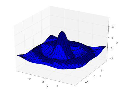
You can now easily produce plots of functions of the form z = f(x,y):

splot(lambda x, y: 10*sinc(hypot(x,y)), [-10,10], [-10,10])


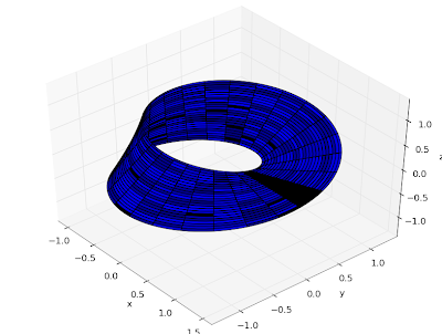
You can just as easily plot more general parametric functions x,y,z = f(u,v). The following plots a Möbius strip:

def f(u,v):
d = (1+0.5*v*cos(0.5*u))
x = d*cos(u)
y = d*sin(u)
z = 0.5*v*sin(0.5*u)
return x,y,z

splot(f, [0,2*pi], [-1,1])


(I'm not sure why there are black spots in the image. This seems to be a matplotlib bug.)

Matrix calculus


It's now possible to compute exponentials, sines, cosines, square roots, logarithms, and complex powers (Az) of square matrices:


>>> mp.dps = 25; mp.pretty = True
>>> A = matrix([[2,3,1+j],[1,0,-1],[2,1,5]])
>>> nprint(expm(A))
[ (27.6034 + 41.2728j) (24.9924 + 31.1189j) (8.67256 + 68.271j)]
[(-15.0962 + 1.51713j) (-10.1713 + 1.30035j) (-28.7003 - 0.401789j)]
[ (125.368 + 37.7417j) (98.9812 + 26.9693j) (158.616 + 85.1593j)]
>>> nprint(logm(expm(A)))
[(2.0 - 5.35398e-26j) (3.0 + 6.9172e-26j) (1.0 + 1.0j)]
[(1.0 + 4.94422e-26j) (4.42102e-25 - 1.14411e-25j) (-1.0 - 1.95948e-27j)]
[(2.0 + 1.58966e-26j) (1.0 - 8.57028e-27j) (5.0 + 3.23653e-27j)]
>>> nprint(sqrtm(A)**2)
[(2.0 - 8.25839e-30j) (3.0 - 8.40399e-30j) (1.0 + 1.0j)]
[(1.0 + 4.63764e-30j) (4.84564e-30 - 3.27721e-31j) (-1.0 + 7.47261e-31j)]
[(2.0 - 4.31871e-30j) (1.0 + 1.78726e-31j) (5.0 + 2.54582e-29j)]
>>> nprint(powm(powm(A,1+j),1/(1+j)))
[(2.0 - 1.12995e-26j) (3.0 - 8.93158e-27j) (1.0 + 1.0j)]
[(1.0 - 1.54352e-26j) (9.23906e-27 - 1.67262e-26j) (-1.0 - 2.62243e-27j)]
[(2.0 + 9.97431e-27j) (1.0 + 1.56341e-26j) (5.0 - 1.79194e-26j)]


The code also works with the double precision fp context, which obviously is much faster for large matrices. When computing square roots and logarithms, most of the time is spent on matrix inversion, which can be accelerated by substituting in numpy:


>>> from mpmath import fp
>>> A = fp.randmatrix(20)
>>> B = fp.sqrtm(A)
>>> timing(fp.sqrtm, A)
3.6470590535948006
>>>
>>> import numpy
>>> fp.inverse = lambda A: fp.matrix(numpy.linalg.inv(A.tolist()))
>>>
>>> timing(fp.sqrtm, A)
1.0815329881311735
>>> C = fp.sqrtm(A)
>>>
>>> fp.mnorm(A-B**2)
3.5001514923930131e-14
>>> fp.mnorm(A-C**2)
2.6462503380426079e-14


It could be much faster still by doing everything in numpy. Probably in the future fp should be improved to seamlessly use numpy internally for all available matrix operations. Patches are welcome!

Borel summation of divergent hypergeometric series


The hypergeometric series of degree p > q+1 are divergent for |z| > 0. Nevertheless, they define asymptotic expansions for analytic functions which exist in the sense of Borel summation. Previously, mpmath knew only how to evaluate 2F0 (whose Borel sum has a closed form), but now it can evaluate the functions of higher degree as well.

To illustrate, the cosine integral Ci(z) has an asymptotic series representation in terms of 3F0:


This representation is efficient for very large values of |z|, where the argument of the hypergeometric series is small. But with z = 0.5, say, the series does not yield a single digit. With a value of z = 10 or so, the series only gives about 3 digits with an optimal truncation:

>>> z = 10.0
>>> for n in range(1,16):
... print sum(rf(0.5,k)*rf(1,k)*rf(1,k)*(-4/(z**2))**k/fac(k) for k in range(n))
...
1.0
0.98
0.9824
0.98168
0.9820832
0.98172032
0.9821993216
0.981327538688
0.9834198176768
0.977017443971072
1.00134646405284
0.888946391275078
1.50939479300832
-2.52351981825774
27.9653146429137


Of course, there are ways to compute the cosine integral using convergent series. But if we pretend that we only know about the asymptotic series, then the Borel regularization means that we can evaluate the function to high precision even for small z:

>>> mp.dps = 25; mp.pretty = True
>>> z = mpf(0.5)
>>> u = -4/z**2
>>> H1 = hyper([1,1,1.5],[],u)
>>> H2 = hyper([0.5,1,1],[],u)
>>>
>>> print log(z)-log(z**2)/2-cos(z)/z**2*H1+sin(z)/z*H2
-0.1777840788066129013358103
>>> print ci(z)
-0.1777840788066129013358103


The z = 10 series above, to high precision:

>>> hyper([0.5,1,1],[],-4/(10.0**2))
0.9819103501017016869905255
>>> mp.dps = 40
>>> hyper([0.5,1,1],[],-4/(10.0**2))
0.9819103501017016869905255431829554224704


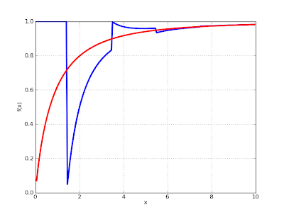
It's instructive to visualize the optimal truncations of an asymptotic series compared to the exact solution. Notice how, for an alternating series like this, the truncations alternate between over- and undershooting:

def optimal_asymp(z):
u = -4/(z**2)
term_prev = inf
s = 0.0
for k in range(30):
term = rf(0.5,k)*rf(1,k)*rf(1,k)*u**k/fac(k)
if abs(term) < abs(term_prev):
s += term
term_prev = term
else:
break
return s

def exact(z):
u = -4/(z**2)
return hyper([0.5,1,1],[],u)

mp.dps = 10
plot([optimal_asymp, exact], [0,10])


The catch with this feature? Computing the Borel regularization involves evaluating (nested) numerical integrals with a hypergeometric function in the integrand. Except for special parameters (where degree reductions happen internally -- the Ci series above happens to be such a case), it's not very fast.

Optional consistency with Mathematica


I often try to follow Mathematica's conventions regarding limits, special values and branch cuts of special functions. This simplifies testing (I can directly compare values with Mathematica), and usually Mathematica's conventions seem well-reasoned.

There are exceptions, however. One such exception concerns Mathematica's interpretation of 2F1(a,b,c,z) for b = c a negative integer. Mathematica interprets this as a polynomial, which doesn't make much sense since the denominator of the zero term is zero. It's not even consistent with how Mathematica evaluates this function for a symbolic variable:

In[3]:= Hypergeometric2F1[3,-2,-2,2]

Out[3]= 31

In[4]:= Hypergeometric2F1[3,b,b,2]

Out[4]= -1


Maybe there is a good reason for doing what Mathematica does, but it's at the very least not documented anywhere. I've now changed mpmath to instead interpret the two parameters as eliminating each other and giving a 1F0 function (which is what Mathematica does for a generic value). The Mathematica-compatible value can be recovered by explicitly disabling parameter elimination:

>>> mp.pretty = True
>>>
>>> hyp2f1(3,-2,-2,2)
-1.0
>>> hyp2f1(3,-2,-2,2,eliminate=False)
31.0


On a related note, I've fixed the Meijer G-function to switch between its z and 1/z forms automatically to follow Mathematica's definition of the function. This introduces discontinuities in the function for certain orders. The user can explicitly choose which form to use (so as to obtain a continuous function) with series=1 or series=2.

Internal reorganization


In a long overdue change, I've moved many of the modules in mpmath into subdirectories. The multiprecision library code is now located in mpmath/libmp; special functions are in mpmath/functions, calculus routines are in mpmath/calculus, and routines for matrices and linear algebra are in mpmath/matrices.

This shouldn't affect any documented interfaces, but it will break external code that directly uses mpmath internal functions. The mpmath interfaces in SymPy and Sage will need some editing for the next version update. The breakage should be straightforward to fix (mostly just a matter of changing imports).

Since the next version of mpmath is definitely going to break some code, I might use the opportunity to do some other cosmetic interface changes as well. Ideally, after the next version, the interface will be stable until and beyond mpmath 1.0 (whenever that happens). But the version number is still at 0.x for a reason -- no compatibility guarantees.

Thursday, January 7, 2010

Accurate hypergeometric functions for large parameters

Holiday season means more free time for coding (yay!). In this commit, I've fixed the remaining major accuracy issues with hypergeometric functions in mpmath. The effect, generally speaking, is that mpmath will now deal much more robustly with large parameters of hypergeometric-type functions.

Previously, you would obtain an accurate value with parameters of magnitude ≈ 10−1 - 101 (say), and often for large parameters as well, but for some functions the accuracy would quickly deteriorate if parameters were increased (or moved closer to singularities). You could still obtain any accuracy by simply increasing the working precision, but you had to manually figure out the amount of extra precision required; the news is that mpmath now automatically gives a value with full accuracy even for large parameters (or screams out loud if it fails to compute an accurate value).

This doesn't mean that you can't trick mpmath into computing a wrong value by choosing sufficiently evil parameters, but it's much harder now than simply plugging in large values. Abnormally large values will now mainly accomplish abnormal slowness (while mpmath implements asymptotic expansions with respect to the argument of hypergeometric functions, evaluation for asymptotically large parameters is a much harder problem as far as I'm aware -- so mpmath in effect accomplishes it by brute force.)

The most trivial change was to change the series summation to aim for control of the relative error instead of the absolute error. This affects alternating series, where large parameters lead to very small function values. Previously, something like the following would happen:


>>> mp.dps=5; hyp1f1(-5000, 1500, 100)
1.6353e-14
>>> mp.dps=15; hyp1f1(-5000, 1500, 100)
8.09813050863682e-25
>>> mp.dps=30; hyp1f1(-5000, 1500, 100)
-1.38318247777802583583082760724e-39


This isn't disastrously bad since the absolute error is controlled (summing this series naively in floating-point arithmetic might give something like 1e+234 due to catastrophic cancellation). But now, you get the relatively accurate answer right away, which is much nicer:


>>> mp.dps = 5; hyp1f1(-5000, 1500, 100)
9.1501e-185
>>> mp.dps = 15; hyp1f1(-5000, 1500, 100)
9.15012134245639e-185
>>> mp.dps = 30; hyp1f1(-5000, 1500, 100)
9.15012134245639443114220499541e-185


Of course, if the value is too small, the evaluation loop must abort eventually. The default behavior now is to raise an exception if relative accuracy cannot be obtained. The user can force a return value by either permitting a higher internal precision before aborting, or specifying a size 2−zeroprec below which the value is small enough to be considered zero:


>>> hyp1f1(-8000, 4000, 1500)
Traceback (most recent call last):
...
ValueError: hypsum() failed to converge to the requested 53 bits of accuracy
using a working precision of 3568 bits. Try with a higher maxprec,
maxterms, or set zeroprec.
>>>
>>>
>>> hyp1f1(-8000, 4000, 1500, maxprec=10000)
4.36754212717293e-1350
>>> hyp1f1(-8000, 4000, 1500, accurate_small=False)
-1.99286380611911e-25
>>> hyp1f1(-8000, 4000, 1500, zeroprec=1000)
0.0


Since exceptions are inconvenient, it will be necessary to add some more symbolic tests for exact zeros for certain functions (particularly orthogonal polynomials) where exact zeros arise as important special cases.

Also, cancellation detection in hypercomb is now the default for all functions. This fixes, among other things, a bug in the Meijer G-function reported by a user via email. Before:


>>> meijerg([[],[]],[[0],[]],0.1)
0.90483741803596
>>> meijerg([[],[]],[[0,0],[]],0.1)
1.47347419562219
>>> meijerg([[],[]],[[0,0,0],[]],0.1)
1.61746025085449
>>> meijerg([[],[]],[[0,0,0,0],[]],0.1) # suspicious
13194139533312.0


After:

>>> meijerg([[],[]],[[0],[]],0.1)
0.90483741803596
>>> meijerg([[],[]],[[0,0],[]],0.1)
1.47347419562219
>>> meijerg([[],[]],[[0,0,0],[]],0.1)
1.61745972140487
>>> meijerg([[],[]],[[0,0,0,0],[]],0.1)
1.56808223438324


Another important change is more correct handling parameters very close to negative integers, particularly those appearing in denominators of series. Previously, unless the integer n was small enough or the precision was set high enough, this situation would yield a bogus value (that of a prematurely truncated series):


>>> n = -20
>>> nh = fadd(n, 1e-100, exact=True)
>>> hyp0f1(n, 0.25) # nonsense
0.987581857511351
>>> hyp0f1(nh, 0.25) # same nonsense
0.987581857511351


Now, correctly:


>>> n = -20
>>> nh = fadd(n, 1e-100, exact=True)
>>> hyp0f1(n, 0.25)
Traceback (most recent call last):
...
ZeroDivisionError: pole in hypergeometric series
>>> hyp0f1(nh, 0.25)
1.85014429040103e+49


Finally, and probably most importantly, the limit evaluation code has been changed to adaptively decrease the size of perturbation until convergence. Under fairly general assumptions, the maximum accurate perturbation at precision p can easily be shown to be 2−(p+C); the problem is that the parameter-dependent constant C isn't generally known. Previously C was just set to a small value (10), and naturally this would break down for some functions when parameters were increased beyond roughly that magnitude.

I briefly considered the idea of estimating C analytically in terms of the parameters, and while I think this can be done rigorously, it seems difficult -- especially to do it tightly (grossly overestimating C would murder performance). The algorithm implemented now is quasi-rigorous, and although there is some slowdown (sometimes by a fair amount), the improved reliability is definitely worth it. A user can also manually supply a perturbation size of their own taste, thereby overriding adaptivity. If the user supplies an intelligent value, this gives both the speed of the old code and full rigor. Probably some intelligent choices for particular functions could be made automatically by mpmath too, to recover the old speed in common cases.

An example of a situation where this becomes necessary is for Legendre functions with certain large parameter combinations. With the old code:

>>> mp.dps = 15; legenp(0.5, 300, 0.25) # bad
4.19317029788723e+626
>>> mp.dps = 30; legenp(0.5, 300, 0.25) # bad
3.72428336871098039162972441784e+611
>>> mp.dps = 60; legenp(0.5, 300, 0.25) # bad
2.93794154954090326636196697693611381787845107728298382876544e+581
>>> mp.dps = 100; legenp(0.5, 300, 0.25) # only accurate to a few digits
-1.71750854949725238788826203712778687036438365374945625996246145924802366061559
6579520831362887006032e+578


With the new code:

>>> mp.dps = 15; legenp(0.5, 300, 0.25)
-1.71750854949725e+578
>>> mp.dps = 30; legenp(0.5, 300, 0.25)
-1.71750854949725238788826203713e+578
>>> mp.dps = 60; legenp(0.5, 300, 0.25)
-1.71750854949725238788826203712778687063419097363472262860567e+578
>>> mp.dps = 15; legenp(0.5, 300, 0.25, hmag=300) # faster, with manual perturbation
-1.71750854949725e+578


Another example is for Bessel functions differentiated to high order. With the old code:

>>> mp.dps = 15; besseli(2, 10, derivative=100) # bad
2.63560662943646e+34
>>> mp.dps = 30; besseli(2, 10, derivative=100) # bad
23408889310840499424.9813614712
>>> mp.dps = 60; besseli(2, 10, derivative=100) # only accurate to a few digits
821.238621006501815018537509753672810563116338269219460709828


With the new code:

>>> mp.dps = 15; besseli(2, 10, derivative=100)
821.238621006483
>>> mp.dps = 30; besseli(2, 10, derivative=100)
821.238621006483348660925541651
>>> mp.dps = 60; besseli(2, 10, derivative=100)
821.238621006483348660925541650744338655411830854860813048862


In related news, I've given all hypergeometric-type functions the ability to accept kwargs and pass them on to hypercomb and hypsum. This means that tuning and error control options will be available for a large number of functions (Bessel functions, etc), which could be useful for some users who need to do advanced calculations. I have yet to document these features thoroughly (the interface will also perhaps be tweaked before the next release).