Thursday, August 13, 2009

Released: mpmath 0.13

I released mpmath 0.13 today. See the announcement for details. Soon coming to a Sage or SymPy near you!

I've blogged extensively about the new features that went into this version over the last two months. The short version of the changelog is "lots of special functions". For convenience, here a list of all posts:


I also suggest a look at the documentation and particularly the special functions section.

Tuesday, August 11, 2009

Torture testing special functions

Today I implemented a set of torture test for special functions in mpmath.

The function torturer takes a function, say f = airyai or f = lambda z: hyp1f1(1.5, -2.25, z), and attempts to evaluate it with z = a · 10n as n ranges between -20 and 20, with a ≈ 1, 1+i, i, -1+i, -1. (The "≈" indicates multiplication by an additional quasi-random factor near unity.)

Thus it tests a wide range of magnitudes (both tiny and huge), with pure positive, negative, imaginary, and complex arguments; i.e. covering most distinct regions of the complex plane. (It doesn't cover the lower half-plane, but that's generally just a waste of time since most function algorithms are agnostic about the sign of the imaginary part -- this should be done for some functions in the future, however.)

Each evaluation is also performed at a range of precisions, between 5 and 150 digits by default (for fast functions the max precision is set much higher). The results at two successive precisions are compared to verify that they agree relatively to the lesser of the precisions (with a single-digit error allowed for roundoff error).

This doesn't guarantee correctness, of course -- I might have implemented the wrong formula for the function -- but it's a strong check that whatever formula has been implemented is being evaluated accurately. It does provide some amount of correctness testing for those functions that use more than one algorithm depending on precision and/or the magnitude of the argument (and this includes the hypergeometric functions). If one algorithm is used at low precision and another at high precision, then an error in either will be revealed when comparing results.

My original intention with was just to check robustness of the asymptotic expansions of hypergeometric functions. Testing with a continuous range of magnitudes ensures that there aren't any regions where convergence gets impossibly slow, a loop fails to terminate, an error estimate is insufficient, etc. (And this needs to be done at several different levels of precision.) I then ended up including many other functions in the list of torture tests as well.

The results? I discovered (and fixed!) some 10-20 bugs in mpmath. Most were of the kind "only 43 accurate digits were returned where 50 were expected" and due to inadequate error estimates and/or insufficient extra precision being allocated (mostly in argument transformations). I actually knew about many of the problems, and had just neglected to fix them because they wouldn't show up for "normal" arguments (and in particular, there weren't any existing tests that failed).

Lesson to be learned: if it isn't tested, it probably doesn't work (fully). Semi-automatic exhaustive or randomized testing (the more "evil" inputs, the better), is a necessary complement to testing hand-picked values.

There is more to be done:


  • Some functions don't yet pass the torture tests

  • Rather than just large/small, the relevant stress measure for some functions is closeness to a negative integer, closeness to the unit circle, etc

  • Functions of more than one argument should be tested with randomly selected values for all parameters


But already now, the torture tests have done a good job. Tellingly, functions I implemented recently are much less buggy than functions I implemented long ago (even just three months ago). Periodically rewriting old code as one learns more is bound to improve quality :-)

Speaking of bugs, Mathematica doesn't pass the mpmath torture test suite (far from it). An example of something that will fail:


In[47]:= N[HypergeometricPFQ[{1},{-1/4,1/3},10^10],15]

General::ovfl: Overflow occurred in computation.

General::ovfl: Overflow occurred in computation.

General::ovfl: Overflow occurred in computation.

General::stop: Further output of General::ovfl
will be suppressed during this calculation.

(... nothing for 5 minutes)

Interrupt> a

Out[47]= $Aborted


And mpmath (instantaneously):


>>> mp.dps = 15; mp.pretty = True
>>> hyp1f2(1,(-1,4),(1,3),10**10)
-3.53521222026601e+86866


By the way, the current set of torture tests takes about 11 minutes to run on my computer with psyco and gmpy (much longer without either). It's possibly a better benchmark than the standard tests.

Update: running the torture tests with multiprocessing on sage.math takes only 28 seconds (which is the time for the slowest individual test). Go parallel!

Sunday, August 9, 2009

3D visualization of complex functions with matplotlib

Hooray! matplotlib 0.99 is out and it has 3D plotting, finally!

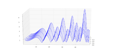
I've shown a lot of color plots of complex functions on this blog to demonstrate complex functions in mpmath. These plots are informative, but sometimes a 3D plot (typically of the function's absolute value) gives a much better view. A big advantage of 3D plots over 2D color plots is that far fewer evaluation points are required for a good high-resolution image, and this helps when visualizing the slower functions in mpmath.

There will probably be a 3D plot function in a future version of mpmath (or two functions; for two-variable real, and complex functions), similar in style to the existing matplotlib wrappers plot and cplot. Until I've figured out the details, I'll share a couple of test plots.

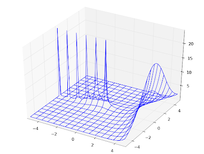
Coulomb wave function of a complex argument, F(6,4,z):


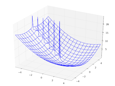
Principal-branch logarithmic gamma function:


Gamma function:


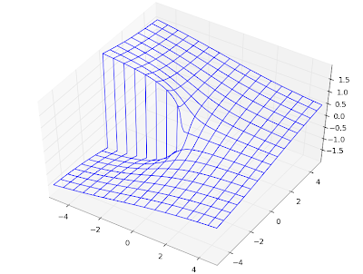
Imaginary part of Lambert W function, 0th branch:


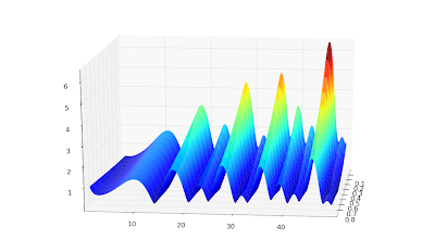
Riemann zeta function in the critical strip:


Those are all wireframe plots. It's also possible to do surface plots. Using the Riemann zeta function again, a surface plot looks as follows:


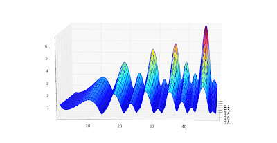
Surface + wireframe plot:


None of these is perfect. I'd like to be able to do a surface plot with a widely spaced wireframe mesh to pronounce the geometry, and smooth colored surface between the meshes. This doesn't seem possible with matplotlib because the surface plot doesn't do smoothing (even with a stride selected); overlaying a wireframe works decently, but the wireframe doesn't render with occlusion and this looks bad for some functions. Since the pure wireframe plot is much faster, I think I prefer it for now.

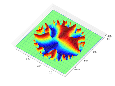
For complex functions, it'd also be nice with a color function separate from the geometry function -- then you could plot the phase as color in the same picture.

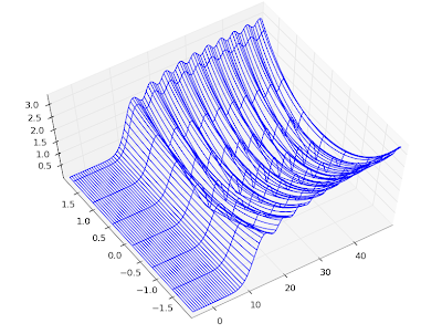
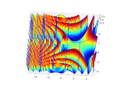
Color helps for visualizing complicated structure, especially for phase plots. Below, I've plotted the phase (actually the sine of the phase, to make it continuous) of a Jacobi theta function θ3(1+4j/3,q) (restricted to |q| < 0.8, because it gets extremely messy for larger |q|):


The phase of the Barnes G-function:


I could do many more, but that will probably enough for this blog :-)

To reproduce any of these, use the following script with trivial modifications. It's a straightforward extension of the example scripts in the matplotlib documentation.


from mpl_toolkits.mplot3d import Axes3D
from matplotlib import cm
import pylab
import numpy as np
import mpmath
mpmath.dps = 5

# Use instead of arg for a continuous phase
def arg2(x):
return mpmath.sin(mpmath.arg(x))

#f = lambda z: abs(mpmath.loggamma(z))
#f = lambda z: arg2(mpmath.exp(z))
#f = lambda z: abs(mpmath.besselj(3,z))
f = lambda z: arg2(mpmath.cos(z))

fig = pylab.figure()
ax = Axes3D(fig)
X = np.arange(-5, 5, 0.125)
Y = np.arange(-5, 5, 0.125)
X, Y = np.meshgrid(X, Y)
xn, yn = X.shape
W = X*0
for xk in range(xn):
for yk in range(yn):
try:
z = complex(X[xk,yk],Y[xk,yk])
w = float(f(z))
if w != w:
raise ValueError
W[xk,yk] = w
except (ValueError, TypeError, ZeroDivisionError):
# can handle special values here
pass
print xk, xn

# can comment out one of these
ax.plot_surface(X, Y, W, rstride=1, cstride=1, cmap=cm.jet)
ax.plot_wireframe(X, Y, W, rstride=5, cstride=5)

pylab.show()

Tuesday, August 4, 2009

Coulomb wave functions and orthogonal polynomials

Work has been a bit slow over the last two weeks, partially due to the fact that I was away during one of them. Nevertheless, I've been able to add a couple of more functions to mpmath, as described in the following post below. With these functions committed, I'm probably going to stop adding features and just do a new release as soon as possible (some documentation and general cleanup will be required first).

Coulomb wave functions

I have, due to a request, implemented the Coulomb wave functions (commit). The Coulomb wave functions are used in quantum physics; they solve the radial part of the Schrödinger equation for a particle in a 1/r potential.

The versions in mpmath are fully general. They work not only for an arbitrarily large or small radius, but for complex values of all parameters. Some example evaluations:


>>> mp.dps = 25; mp.pretty = True
>>> coulombf(4, 2.5, 1000000)
-0.9713831935409625197404938
>>> coulombf(2+3j, 1+j, 100j)
(2.161557009297068729111076e+37 + 1.217455850269101085622437e+39j)
>>> coulombg(-3.5, 2, '1e-100')
2.746460651456730226435998e+252


The definitions of the Coulomb wave functions for complex parameters are based mostly on this paper by N. Michel, which describes a special-purpose C++ implementation. I'm not aware of any other software that implements Coulomb wave functions, except for GSL which only supports limited domains in fixed precision.

The Coulomb wave functions are numerically difficult to calculate: the canonical representation requires complex arithmetic, and the terms vary by many orders of magnitude even for small parameter values. Arbitrary-precision arithmetic, therefore, is almost necessary even to obtain low-precision values, unless one uses much more specialized evaluation methods. The current mpmath versions are simple and robust, although they can be fairly slow in worst cases (i.e. when they need to use a high internal precision). Timings for average/good cases are in the millisecond range,


>>> timing(coulombf, 3, 2, 10)
0.0012244852348553437
>>> timing(coulombg, 3, 2, 10)
0.0068572681723514609


but they can climb up towards a second or so when large cancellations occur. Someone who needs faster Coulomb wave functions, say for a limited range of parameters, could perhaps find mpmath useful for testing a more specialized implementation against.

The speed is plenty for basic visualization purposes. Below I've recreated graphs 14.1, 14.2 and 14.5 from Abramowitz & Stegun.


mp.dps = 5

# Figure 14.1
F1 = lambda x: coulombf(x,1,10)
F2 = lambda x: coulombg(x,1,10)
plot([F1,F2], [0,15], [-1.2, 1.7])

# Figure 14.3
F1 = lambda x: coulombf(0,0,x)
F2 = lambda x: coulombf(0,1,x)
F3 = lambda x: coulombf(0,5,x)
F4 = lambda x: coulombf(0,10,x)
F5 = lambda x: coulombf(0,x/2,x)
plot([F1,F2,F3,F4,F5], [0,25], [-1.2,1.6])

# Figure 14.5
F1 = lambda x: coulombg(0,0,x)
F2 = lambda x: coulombg(0,1,x)
F3 = lambda x: coulombg(0,5,x)
F4 = lambda x: coulombg(0,10,x)
F5 = lambda x: coulombg(0,x/2,x)
plot([F1,F2,F3,F4,F5], [0,30], [-2,2])


Also, a plot for complex values, cplot(lambda z: coulombg(1+j, -0.5, z)):


Orthogonal polynomials

I've added the (associated) Legendre functions of the first and second kind, Gegenbauer, (associated) Laguerre and Hermite functions (commits 1, 2, 3, 4). This means that mpmath finally supports all the classical orthogonal polynomials. As usual, they work in generalized form, for complex values of all parameters.

A fun thing to do is to verify orthogonality of the orthogonal polynomials using numerical quadrature:

>>> mp.dps = 15
>>> chop(quad(lambda t: exp(-t)*t**2*laguerre(3,2,t)*laguerre(4,2,t), [0,inf]))
0.0
>>> chop(quad(lambda t: exp(-t**2)*hermite(3,t)*hermite(4,t), [-inf,inf]))
0.0


As another basic demonstration, here are some Legendre functions of the second kind, visualized:
F1 = lambda x: legenq(0,0,x)
F2 = lambda x: legenq(1,0,x)
F3 = lambda x: legenq(2,0,x)
F4 = lambda x: legenq(3,0,x)
F5 = lambda x: legenq(4,0,x)
plot([F1,F2,F3,F4,F5], [-1,1], [-1.3,1.3])


Implementing these functions is a lot of work, I've found. The general case is simple (just fall back to generic hypergeometric code), but the special cases (singularities, limits, asymptotically large arguments) are easy to get wrong and there are lots of them to test and document.

My general methodology is to implement the special functions as the Wolfram Functions site defines them (if they are listed there), test my implementation against exact formulas, and then test numerical values against Mathematica. Unfortunately, Wolfram Functions often leaves limits undefined, and is not always consistent with Mathematica. In fact, Mathematica is not even consistent with itself. Consider the following:


In[277]:= LaguerreL[-1, b, z] // FunctionExpand

Out[277]= 0

In[278]:= LaguerreL[-1, -2, z] // FunctionExpand

z 2
E z
Out[278]= -----
2


It's tempting to just leave such a case undefined in mpmath and move on (and perhaps fix it later if it turns out to be used). Ideally mpmath should handle all singular cases correctly and consistently, and it should state in the documentation precisely what it will calculate for any given input so that the user doesn't have to guess. Testing and documenting special cases is very time-consuming, however, and although I'm making progress, this work is far from complete.