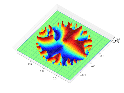
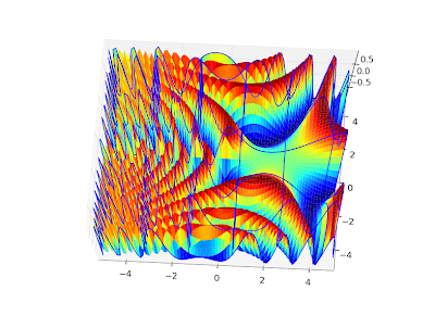
Tuesday, December 22, 2009

Analytic continuation of 3F2, 4F3 and higher functions

As of a recent commit, mpmath can evaluate the analytic continuation of the generalized hypergeometric function p+1Fp for any p. Previously 2F1 (the Gaussian hypergeometric function) was supported -- see earlier blog posts -- but not 3F2 and higher. This addition means that the generalized hypergeometric function is finally supported essentially everywhere where it is "well-posed" (in the sense that the series has nonzero radius of convergence), so it is a rather significant improvement. Unfortunately, the implementation is still not perfect, but I decided to commit the existing code since it is quite useful already (and long overdue).

As proof of operation, I deliver plots of 3F2 and 4F3, requiring both |z| < 1 and |z| > 1:

from mpmath import *
f1 = lambda z: hyp3f2(1,2,3,4,5,z)
f2 = lambda z: hyper([1,2,3,4],[5,6,7],z)
plot([f1,f2], [-2,2])


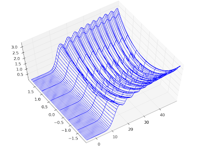
A portrait of 3F2 restricted to the unit circle:

plot(lambda x: hyp3f2(1,2,3,4,5,exp(2*pi*j*x)), [-1,1])


A numerical value of 5F4 with z on the unit circle, with general complex parameters:

>>> mp.dps = 50
>>> print hyper([1+j,0.5,-2j,1,0.5+0.5j],[0.5j,0.25,-j,-1-j],-1)
(-1.8419705729324526212110109087877199070037836117341 -
0.57799141426978758652682670969879368618437786161612j)


High precision values of 3F2 at z = 1 and z = 1 + ε:

>>> print hyp3f2(1,1,2,3.5,1.5,1)
2.2603241503205748814116375624327119385797950825522
>>> print hyp3f2(1,1,2,3.5,1.5,'1.0001')
(2.2626812356987790952469291649495098300894035980837 -
0.00092505569713084902188662960467216683326695892509251j)


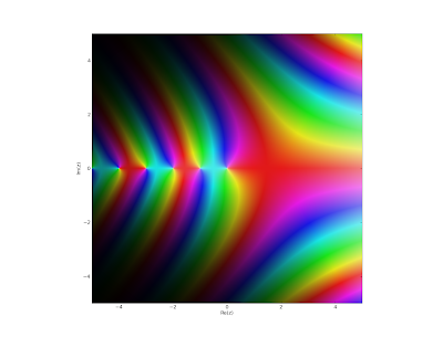
A complex plot of 3F2:

>>> mp.dps = 5
>>> cplot(lambda z: hyp3f2(2.5,3,4,1,2.25,z), [-2,2], [-2,2],
... points=50000)


A bit of theoretical background: the hypergeometric series pFq has an infinite radius of convergence when p ≤ q, so it can in principle be evaluated then by adding sufficiently many terms at sufficiently high precision (although in practice asymptotic expansions must be used for large arguments, as mpmath does). In the balanced case when p = q+1, i.e. for 1F0(a,z), 2F1(a,b,c,z), 3F2(...), 4F3(...), ..., the series converges only when |z| < 1 (plus in some special instances). This is due to the fact that the hypergeometric function has a singularity (a pole or branch point, depending on parameters) at z = 1, in turn owing to the fact that the hypergeometric differential equation is singular at z = 1. (The reason that the p = q+1 and not p = q case is "balanced" is that there is an extra, implicit factorial in the hypergeometric series.)

The main ingredient of the analytic continuation of p+1Fp is the inversion formula which replaces z with 1/z and thus handles |z| > 1. This was easy to implement -- the only complication is that integer parameters result in singular gamma factors, but the mechanisms to handle those automatically were already in place. There was no particular reason why I hadn't added that code already.

The tricky part is the unit circle, and the close vicinity thereof, where neither series converges (quickly). I've been looking for good ways handle this, with mixed results.

When I posed the problem on this blog several months back, a reader suggested this paper by Wolfgang Bühring which gives a series for the analytic continuation around z = 1. My finding from trying to implement it is that the rate of convergence of the series generally is poor, and therefore it is not immediately effective for computation. However, convergence acceleration with nsum improves the situation considerably in many cases. Some parameter combinations render the convergence acceleration useless, but even then, it can give a few correct digits, so it is better than nothing (although the implementation should probably warn the user when the result probably is inaccurate). I'm unfortunately not aware of any parameter transformations that would substantially improve convergence. The current implementation uses this method for 3F2 when |z-1| is small; it should work for 4F3 and higher too, but the series coefficients are much more complicated (involving multiply nested sums), so that's yet to be done.

For the rest of the unit circle, I've settled for simply using convergence acceleration directly. This essentially just amounts to passing the hypergeometric series to nsum, which applies Richardson extrapolation and iterated Shanks transformations. The Shanks transformation is actually perfect for this -- it's almost tailor made for convergence acceleration of the balanced hypergeometric series -- and is able to sum the series even outside the circle of convergence, using just a few terms. This covers most of the unit circle -- the catch is just that the acceleration asymptotically deteriorates and ultimately becomes useless close to z = 1, so complementary method (such as the Bühring's is still required there).

Mathematica seems to support unit-circle evaluation of hypergeometric functions quite well. Unfortunately, I don't know how it does it. According to Wolfram's Some Notes On Internal Implementation page,


The hypergeometric functions use functional equations, stable recurrence relations, series expansions, asymptotic series and Padé approximants. Methods from NSum and NIntegrate are also sometimes used.


This looks similar to what I'm doing -- high order Padé approximants and Mathematica's NSum should be equivalent to the nsum-based series acceleration in mpmath. But probably Mathematica employs some more tricks as well.

I've also tested direct integration of the hypergeometric differential equation and of Mellin-Barnes integral representations, but these approaches don't seem to work much better (at least not without many improvments), and at best seem to be relatively slow.

Thursday, September 10, 2009

Python floats and other unusual things spotted in mpmath

I've just put up a branch (named "mp4") containing changes to mpmath that I've been working on for several days now. This branch includes some rather large changes, including support for fixed-precision (machine-precision) arithmetic, and a new implementation of the multiprecision type. The code is a bit rough at the moment, and not all changes are final, so don't expect this in a release in the immediate future.

New mpf implementation


The mp4 branch uses a new mpf type that handles both real and complex values. It makes complex arithmetic quite a bit faster (up to twice the speed), although real arithmetic is a little slower. Some of the slowdown is due to wrapping old-format functions instead of providing new ones, so there is a bit of unnecessary overhead. The biggest advantage is not that the implementation becomes faster, but that it becomes simpler. For example, a nice feature is that complex calculations that yield real results don't need to be converted back to a real type manually. Unfortunately, writing code that also supports Python float and complex (see below) somewhat reduce the usefulness of such features.

Imaginary infinities are a little more well-behaved (i.e. j*(j*inf) gives -inf and not a complex NaN), and the representation is flexible enough that it might be possible to support unsigned infinities, infinities with an arbitrary complex sign, and possibly even zero with an arbitrary complex sign -- hey, perhaps infinities and zeros with order and residue information attached to them so you can evaluate gamma(-3)**2 / gamma(-5) / gamma(-2) directly? (Well, I'm not sure if this is actually possible, and if it is, it's probably way overkill :-)

This new implementation will not necessarily make it -- it depends on whether the pros outweigh the cons. I would very much appreciate review by others. Regardless of the outcome, writing it has been very useful for identifying and fixing problems in the interface between "low level" and "high level" code in mpmath.

This should particularly simplify the future support for a C or Cython-based backend. In fact, the current fixed-precision backend (see below) only uses about 200 lines of code -- and although it's not complete yet, it handles a large set of calculations. Adding a fast multiprecision backend based on Sage or GMPY can probably be done in an evening now. I'm not going to do such a thing right now, as I want to fix up the existing code before adding anything new; should someone else be interested though, then by all means go ahead.

I've also inserted a few other optimizations. As noted before on this blog, many of the special functions in mpmath are evaluated as linear combinations of hypergeometric series. All those functions basically fall back to a single routine which sums hypergeometric series. The mp4 branch contains a new implementation of this routine that is up to about twice as fast as before. The speed is achieved by code generation: for every different "type" (degree, parameter types) of hypergeometric series, a specialized version is generated with various bookkeeping done in advance so it doesn't have to be repeated in every iteration of the inner loop.

As an example, the following runs at 1.7x the speed:

>>> 1/timing(mpmath.hyp1f1, 1.5, 2.2, 1.35)
5620.8844813722862
>>> 1/timing(mp4.hyp1f1, 1.5, 2.2, 1.35)
9653.1737629459149


Nearly all tests pass with the new mpf type used instead of the old one -- the only significant missing piece is interval arithmetic.

Fixed-precision arithmetic


Several people have requested support for working with regular Python floats and complexes in mpmath. Often you only need a few digits of accuracy, and mpmath's multiprecision arithmetic is unnecessarily slow. Many (though not all) of the algorithms in mpmath work well in fixed precision; the main problem with supporting this feature has been that of providing an appropriate interface that avoids cluttering the code.

In the mp4 branch, this is solved by adding a fixed-precision context. This context uses the same "high-level" methods for special functions, calculus, linear algebra, etc, as the multiprecision context, while low-level functions are replaced with fixed-precision versions. For example exp is just a wrapper around math.exp and cmath.exp.

While the default multiprecision context instance is called mp, the default fixed-precision context instance is called fp. So:


>>> from mp4 import mp, fp
>>> mp.pretty = True
>>> mp.sqrt(-5); type(_)
2.23606797749979j
<class 'mp4.ctx_mp.mpf'>
>>> fp.sqrt(-5); type(_)
2.2360679774997898j
<type 'complex'>


The fixed-precision context is still missing a lot of low-level functions, so many things don't work yet. Let's try a couple of calculations that do work and see how they compare.

Lambert W function


The Lambert W function was the first nontrivial function I tried to get working, since it's very useful in fixed precision and its calculation only requires simple functions. The lambertw method is the same for mp as for fp; the latter just uses float or complex for the arithmetic.


>>> mp.lambertw(7.5)
1.56623095378239
>>> mp.lambertw(3+4j)
(1.28156180612378 + 0.533095222020971j)
>>> fp.lambertw(7.5)
1.5662309537823875
>>> fp.lambertw(3+4j)
(1.2815618061237759+0.53309522202097104j)

The fixed-precision results are very accurate, which is not surprising since the Lambert W function is implemented using a "self-correcting" convergent iteration. In fact, the multiprecision implementation could be sped up by using the fixed-precision version to generate the initial value. The speed difference is quite striking:

>>> 1/timing(mp.lambertw, 7.5)
1249.5319808144905
>>> 1/timing(mp.lambertw, 3+4j)
603.49697841726618
>>> 1/timing(fp.lambertw, 7.5)
36095.559380378654
>>> 1/timing(fp.lambertw, 3+4j)
20281.934235976787

Both the real and complex versions are about 30x faster in fixed precision.

Hurwitz zeta function


The Hurwitz zeta function is implemented mainly using Euler-Maclaurin summation. The main ingredients are Bernoulli numbers and the powers in the truncated L-series. Bernoulli numbers are cached, and can be computed relatively quickly to begin with, so they're not much to worry about. In fact, I implemented fixed-precision Bernoulli numbers by wrapping the arbitrary-precision routine for them, so they are available to full 53-bit accuracy. As it turns out, the fixed-precision evaluation achieves nearly full accuracy:


>>> mp.hurwitz(3.5, 2.25); fp.hurwitz(3.5, 2.25)
0.0890122424923889
0.089012242492388816
>>> t1=timing(mp.hurwitz,3.5,2.25); t2=timing(fp.hurwitz,3.5,2.25); 1/t1; 1/t2; t1/t2
473.66504799548278
7008.0267335004173
14.7953216374269


There is a nice 15x speedup, and it gets even better if we try complex values. Let's evaluate the the zeta function on the critical line 0.5+ti for increasing values of t:


>>> s=0.5+10j
>>> mp.hurwitz(s); fp.hurwitz(s)
(1.54489522029675 - 0.115336465271273j)
(1.5448952202967554-0.11533646527127067j)
>>> t1=timing(mp.hurwitz,s); t2=timing(fp.hurwitz,s); 1/t1; 1/t2; t1/t2
213.37891598750548
4391.4815202596583
20.580672180923461

>>> s=0.5+1000j
>>> mp.hurwitz(s); fp.hurwitz(s)
(0.356334367194396 + 0.931997831232994j)
(0.35633436719476846+0.93199783123336344j)
>>> t1=timing(mp.hurwitz,s); t2=timing(fp.hurwitz,s); 1/t1; 1/t2; t1/t2
8.1703453931669383
352.54843617352128
43.149759185011469

>>> s = 0.5+100000j
>>> mp.hurwitz(s); fp.hurwitz(s)
(1.07303201485775 + 5.7808485443635j)
(1.0730320148426455+5.7808485443942352j)
>>> t1=timing(mp.hurwitz,s); t2=timing(fp.hurwitz,s); 1/t1; 1/t2; t1/t2
0.17125208455924443
9.2754935956407891
54.162806949260492


It's definitely possible to go up to slightly larger heights still. The Euler-Maclaurin truncation in the Hurwitz zeta implementation is not really tuned, and certainly has not been tuned for fixed precision, so the speed can probably be improved.

Hypergeometric functions


Implementing hypergeometric series in fixed precision was trivial. That the multi-precision implementation is actually quite fast can be seen by comparing direct evaluations:


>>> mp.hyp1f1(2.5, 1.2, -4.5)
-0.0164674858506064
>>> fp.hyp1f1(2.5, 1.2, -4.5)
-0.016467485850591584
>>> 1/timing(mp.hyp1f1, 2.5, 1.2, -4.5)
6707.6667199744124
>>> 1/timing(fp.hyp1f1, 2.5, 1.2, -4.5)
12049.135305946565


The float version is only about twice as fast. Unfortunately, hypergeometric series suffer from catastrophic cancellation in fixed precision, as can be seen by trying a larger argument:


>>> mp.hyp1f1(2.5, 1.2, -30.5)
6.62762709628679e-5
>>> fp.hyp1f1(2.5, 1.2, -30.5)
-0.012819333651375751


Potentially, checks could be added so that the fixed-precision series raises an exception or falls back to arbitrary-precision arithmetic internally when catastrophic cancellation occurs. However, it turns out that this evaluation works for even larger arguments when the numerically stable asymptotic series kicks in:


>>> mp.hyp1f1(2.5, 1.2, -300.5)
1.79669541078302e-7
>>> fp.hyp1f1(2.5, 1.2, -300.5+0j)
1.7966954107830195e-07


The reason I used a complex argument is that the asymptotic series uses complex arithmetic internally, and Python has an annoying habit of raising exceptions when performing complex-valued operations involving floats (a proper workaround will have to be added). In this case the speedup is close to an order of magnitude:


>>> 1/timing(mp.hyp1f1, 2.5, 1.2, -300.5)
532.36666412814452
>>> 1/timing(fp.hyp1f1, 2.5, 1.2, -300.5+0j)
4629.4746136865342


Another example, a Bessel function. This function is calculated using a hypergeometric series and also a couple of additional factors, so the speedup is quite large:


>>> mp.besselk(2.5, 7.5)
0.000367862846522012
>>> fp.besselk(2.5, 7.5)
0.00036786284652201188
>>> 1/timing(mp.besselk, 2.5, 7.5)
3410.5578142787444
>>> 1/timing(fp.besselk, 2.5, 7.5)
21879.520083463747


The fixed-precision context does not yet handle cancellation of singularities in hypergeometric functions. This can be implemented as in the multiprecision case by perturbing values, although accuracy will be quite low (at best 5-6 digits; sometimes an accurate result will be impossible to obtain).

Numerical calculus


Root-finding works, as does numerical integration, with nice speedups:


>>> fp.quad(lambda x: fp.cos(x), [2, 5])
-1.8682217014888205
>>> mp.quad(lambda x: mp.cos(x), [2, 5])
-1.86822170148882
>>> 1/timing(fp.quad, lambda x: fp.cos(x), [2, 5])
1368.3622602114056
>>> 1/timing(mp.quad, lambda x: mp.cos(x), [2, 5])
55.480651962846274

>>> fp.findroot(lambda x: fp.cos(x), 2)
1.5707963267948966
>>> mp.findroot(lambda x: mp.cos(x), 2)
1.5707963267949
>>> 1/timing(fp.findroot, lambda x: fp.cos(x), 2)
19160.822293284604
>>> 1/timing(mp.findroot, lambda x: mp.cos(x), 2)
1039.4805452292442


The tests above use well-behaved object functions; some corner cases are likely fragile at this point. I also know, without having tried, that many other calculus functions utterly don't work in fixed precision (not by algorithm, nor by implementation). Some work will be needed to support them even partially. At minimum, several functions will have to be changed to use an epsilon of 10-5 or so since full 15-16-digit accuracy requires extra working precision which just isn't available.

Plotting


The plot methods work, and are of course way faster in fixed-precision mode. For your enjoyment, here is the gamma function in high resolution; the following image took only a few seconds to generate:

>>> fp.cplot(fp.gamma, points=400000)


With the default number of points (fp.cplot(fp.gamma)), it's of course instantaneous.

Thursday, August 13, 2009

Released: mpmath 0.13

I released mpmath 0.13 today. See the announcement for details. Soon coming to a Sage or SymPy near you!

I've blogged extensively about the new features that went into this version over the last two months. The short version of the changelog is "lots of special functions". For convenience, here a list of all posts:


I also suggest a look at the documentation and particularly the special functions section.

Tuesday, August 11, 2009

Torture testing special functions

Today I implemented a set of torture test for special functions in mpmath.

The function torturer takes a function, say f = airyai or f = lambda z: hyp1f1(1.5, -2.25, z), and attempts to evaluate it with z = a · 10n as n ranges between -20 and 20, with a ≈ 1, 1+i, i, -1+i, -1. (The "≈" indicates multiplication by an additional quasi-random factor near unity.)

Thus it tests a wide range of magnitudes (both tiny and huge), with pure positive, negative, imaginary, and complex arguments; i.e. covering most distinct regions of the complex plane. (It doesn't cover the lower half-plane, but that's generally just a waste of time since most function algorithms are agnostic about the sign of the imaginary part -- this should be done for some functions in the future, however.)

Each evaluation is also performed at a range of precisions, between 5 and 150 digits by default (for fast functions the max precision is set much higher). The results at two successive precisions are compared to verify that they agree relatively to the lesser of the precisions (with a single-digit error allowed for roundoff error).

This doesn't guarantee correctness, of course -- I might have implemented the wrong formula for the function -- but it's a strong check that whatever formula has been implemented is being evaluated accurately. It does provide some amount of correctness testing for those functions that use more than one algorithm depending on precision and/or the magnitude of the argument (and this includes the hypergeometric functions). If one algorithm is used at low precision and another at high precision, then an error in either will be revealed when comparing results.

My original intention with was just to check robustness of the asymptotic expansions of hypergeometric functions. Testing with a continuous range of magnitudes ensures that there aren't any regions where convergence gets impossibly slow, a loop fails to terminate, an error estimate is insufficient, etc. (And this needs to be done at several different levels of precision.) I then ended up including many other functions in the list of torture tests as well.

The results? I discovered (and fixed!) some 10-20 bugs in mpmath. Most were of the kind "only 43 accurate digits were returned where 50 were expected" and due to inadequate error estimates and/or insufficient extra precision being allocated (mostly in argument transformations). I actually knew about many of the problems, and had just neglected to fix them because they wouldn't show up for "normal" arguments (and in particular, there weren't any existing tests that failed).

Lesson to be learned: if it isn't tested, it probably doesn't work (fully). Semi-automatic exhaustive or randomized testing (the more "evil" inputs, the better), is a necessary complement to testing hand-picked values.

There is more to be done:


  • Some functions don't yet pass the torture tests

  • Rather than just large/small, the relevant stress measure for some functions is closeness to a negative integer, closeness to the unit circle, etc

  • Functions of more than one argument should be tested with randomly selected values for all parameters


But already now, the torture tests have done a good job. Tellingly, functions I implemented recently are much less buggy than functions I implemented long ago (even just three months ago). Periodically rewriting old code as one learns more is bound to improve quality :-)

Speaking of bugs, Mathematica doesn't pass the mpmath torture test suite (far from it). An example of something that will fail:


In[47]:= N[HypergeometricPFQ[{1},{-1/4,1/3},10^10],15]

General::ovfl: Overflow occurred in computation.

General::ovfl: Overflow occurred in computation.

General::ovfl: Overflow occurred in computation.

General::stop: Further output of General::ovfl
will be suppressed during this calculation.

(... nothing for 5 minutes)

Interrupt> a

Out[47]= $Aborted


And mpmath (instantaneously):


>>> mp.dps = 15; mp.pretty = True
>>> hyp1f2(1,(-1,4),(1,3),10**10)
-3.53521222026601e+86866


By the way, the current set of torture tests takes about 11 minutes to run on my computer with psyco and gmpy (much longer without either). It's possibly a better benchmark than the standard tests.

Update: running the torture tests with multiprocessing on sage.math takes only 28 seconds (which is the time for the slowest individual test). Go parallel!

Sunday, August 9, 2009

3D visualization of complex functions with matplotlib

Hooray! matplotlib 0.99 is out and it has 3D plotting, finally!

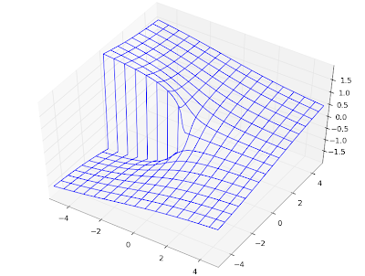
I've shown a lot of color plots of complex functions on this blog to demonstrate complex functions in mpmath. These plots are informative, but sometimes a 3D plot (typically of the function's absolute value) gives a much better view. A big advantage of 3D plots over 2D color plots is that far fewer evaluation points are required for a good high-resolution image, and this helps when visualizing the slower functions in mpmath.

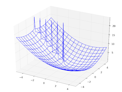
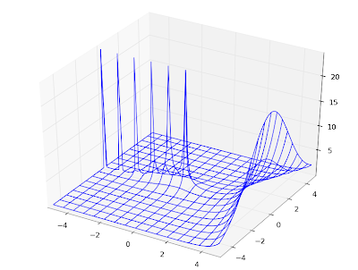
There will probably be a 3D plot function in a future version of mpmath (or two functions; for two-variable real, and complex functions), similar in style to the existing matplotlib wrappers plot and cplot. Until I've figured out the details, I'll share a couple of test plots.

Coulomb wave function of a complex argument, F(6,4,z):


Principal-branch logarithmic gamma function:


Gamma function:


Imaginary part of Lambert W function, 0th branch:


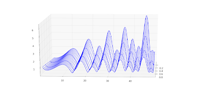
Riemann zeta function in the critical strip:


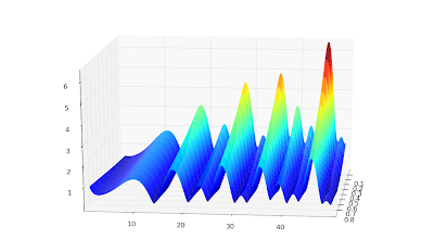
Those are all wireframe plots. It's also possible to do surface plots. Using the Riemann zeta function again, a surface plot looks as follows:


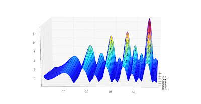
Surface + wireframe plot:


None of these is perfect. I'd like to be able to do a surface plot with a widely spaced wireframe mesh to pronounce the geometry, and smooth colored surface between the meshes. This doesn't seem possible with matplotlib because the surface plot doesn't do smoothing (even with a stride selected); overlaying a wireframe works decently, but the wireframe doesn't render with occlusion and this looks bad for some functions. Since the pure wireframe plot is much faster, I think I prefer it for now.

For complex functions, it'd also be nice with a color function separate from the geometry function -- then you could plot the phase as color in the same picture.

Color helps for visualizing complicated structure, especially for phase plots. Below, I've plotted the phase (actually the sine of the phase, to make it continuous) of a Jacobi theta function θ3(1+4j/3,q) (restricted to |q| < 0.8, because it gets extremely messy for larger |q|):


The phase of the Barnes G-function:


I could do many more, but that will probably enough for this blog :-)

To reproduce any of these, use the following script with trivial modifications. It's a straightforward extension of the example scripts in the matplotlib documentation.


from mpl_toolkits.mplot3d import Axes3D
from matplotlib import cm
import pylab
import numpy as np
import mpmath
mpmath.dps = 5

# Use instead of arg for a continuous phase
def arg2(x):
return mpmath.sin(mpmath.arg(x))

#f = lambda z: abs(mpmath.loggamma(z))
#f = lambda z: arg2(mpmath.exp(z))
#f = lambda z: abs(mpmath.besselj(3,z))
f = lambda z: arg2(mpmath.cos(z))

fig = pylab.figure()
ax = Axes3D(fig)
X = np.arange(-5, 5, 0.125)
Y = np.arange(-5, 5, 0.125)
X, Y = np.meshgrid(X, Y)
xn, yn = X.shape
W = X*0
for xk in range(xn):
for yk in range(yn):
try:
z = complex(X[xk,yk],Y[xk,yk])
w = float(f(z))
if w != w:
raise ValueError
W[xk,yk] = w
except (ValueError, TypeError, ZeroDivisionError):
# can handle special values here
pass
print xk, xn

# can comment out one of these
ax.plot_surface(X, Y, W, rstride=1, cstride=1, cmap=cm.jet)
ax.plot_wireframe(X, Y, W, rstride=5, cstride=5)

pylab.show()

Tuesday, August 4, 2009

Coulomb wave functions and orthogonal polynomials

Work has been a bit slow over the last two weeks, partially due to the fact that I was away during one of them. Nevertheless, I've been able to add a couple of more functions to mpmath, as described in the following post below. With these functions committed, I'm probably going to stop adding features and just do a new release as soon as possible (some documentation and general cleanup will be required first).

Coulomb wave functions

I have, due to a request, implemented the Coulomb wave functions (commit). The Coulomb wave functions are used in quantum physics; they solve the radial part of the Schrödinger equation for a particle in a 1/r potential.

The versions in mpmath are fully general. They work not only for an arbitrarily large or small radius, but for complex values of all parameters. Some example evaluations:


>>> mp.dps = 25; mp.pretty = True
>>> coulombf(4, 2.5, 1000000)
-0.9713831935409625197404938
>>> coulombf(2+3j, 1+j, 100j)
(2.161557009297068729111076e+37 + 1.217455850269101085622437e+39j)
>>> coulombg(-3.5, 2, '1e-100')
2.746460651456730226435998e+252


The definitions of the Coulomb wave functions for complex parameters are based mostly on this paper by N. Michel, which describes a special-purpose C++ implementation. I'm not aware of any other software that implements Coulomb wave functions, except for GSL which only supports limited domains in fixed precision.

The Coulomb wave functions are numerically difficult to calculate: the canonical representation requires complex arithmetic, and the terms vary by many orders of magnitude even for small parameter values. Arbitrary-precision arithmetic, therefore, is almost necessary even to obtain low-precision values, unless one uses much more specialized evaluation methods. The current mpmath versions are simple and robust, although they can be fairly slow in worst cases (i.e. when they need to use a high internal precision). Timings for average/good cases are in the millisecond range,


>>> timing(coulombf, 3, 2, 10)
0.0012244852348553437
>>> timing(coulombg, 3, 2, 10)
0.0068572681723514609


but they can climb up towards a second or so when large cancellations occur. Someone who needs faster Coulomb wave functions, say for a limited range of parameters, could perhaps find mpmath useful for testing a more specialized implementation against.

The speed is plenty for basic visualization purposes. Below I've recreated graphs 14.1, 14.2 and 14.5 from Abramowitz & Stegun.


mp.dps = 5

# Figure 14.1
F1 = lambda x: coulombf(x,1,10)
F2 = lambda x: coulombg(x,1,10)
plot([F1,F2], [0,15], [-1.2, 1.7])

# Figure 14.3
F1 = lambda x: coulombf(0,0,x)
F2 = lambda x: coulombf(0,1,x)
F3 = lambda x: coulombf(0,5,x)
F4 = lambda x: coulombf(0,10,x)
F5 = lambda x: coulombf(0,x/2,x)
plot([F1,F2,F3,F4,F5], [0,25], [-1.2,1.6])

# Figure 14.5
F1 = lambda x: coulombg(0,0,x)
F2 = lambda x: coulombg(0,1,x)
F3 = lambda x: coulombg(0,5,x)
F4 = lambda x: coulombg(0,10,x)
F5 = lambda x: coulombg(0,x/2,x)
plot([F1,F2,F3,F4,F5], [0,30], [-2,2])


Also, a plot for complex values, cplot(lambda z: coulombg(1+j, -0.5, z)):


Orthogonal polynomials

I've added the (associated) Legendre functions of the first and second kind, Gegenbauer, (associated) Laguerre and Hermite functions (commits 1, 2, 3, 4). This means that mpmath finally supports all the classical orthogonal polynomials. As usual, they work in generalized form, for complex values of all parameters.

A fun thing to do is to verify orthogonality of the orthogonal polynomials using numerical quadrature:

>>> mp.dps = 15
>>> chop(quad(lambda t: exp(-t)*t**2*laguerre(3,2,t)*laguerre(4,2,t), [0,inf]))
0.0
>>> chop(quad(lambda t: exp(-t**2)*hermite(3,t)*hermite(4,t), [-inf,inf]))
0.0


As another basic demonstration, here are some Legendre functions of the second kind, visualized:
F1 = lambda x: legenq(0,0,x)
F2 = lambda x: legenq(1,0,x)
F3 = lambda x: legenq(2,0,x)
F4 = lambda x: legenq(3,0,x)
F5 = lambda x: legenq(4,0,x)
plot([F1,F2,F3,F4,F5], [-1,1], [-1.3,1.3])


Implementing these functions is a lot of work, I've found. The general case is simple (just fall back to generic hypergeometric code), but the special cases (singularities, limits, asymptotically large arguments) are easy to get wrong and there are lots of them to test and document.

My general methodology is to implement the special functions as the Wolfram Functions site defines them (if they are listed there), test my implementation against exact formulas, and then test numerical values against Mathematica. Unfortunately, Wolfram Functions often leaves limits undefined, and is not always consistent with Mathematica. In fact, Mathematica is not even consistent with itself. Consider the following:


In[277]:= LaguerreL[-1, b, z] // FunctionExpand

Out[277]= 0

In[278]:= LaguerreL[-1, -2, z] // FunctionExpand

z 2
E z
Out[278]= -----
2


It's tempting to just leave such a case undefined in mpmath and move on (and perhaps fix it later if it turns out to be used). Ideally mpmath should handle all singular cases correctly and consistently, and it should state in the documentation precisely what it will calculate for any given input so that the user doesn't have to guess. Testing and documenting special cases is very time-consuming, however, and although I'm making progress, this work is far from complete.

Wednesday, July 15, 2009

Hurwitz zeta function, Dirichlet L-series, Appell F1

I've added three more functions to mpmath since the last blog update: the Hurwitz zeta function, Dirichlet L-series and the Appell hypergeometric function.

Hurwitz zeta function


The Hurwitz zeta function is available with the syntax hurwitz(s, a=1, derivative=0). It's a separate function from zeta for various reasons (one being to make the plain zeta function as simple as possible). With the optional third argument, it not only computes values, but arbitrarily high derivatives with respect to s (more on which later).

It's quite fast at high precision; e.g. the following evaluation takes just 0.25 seconds (0.6 seconds from cold cache) on my laptop:


>>> mp.dps = 1000
>>> hurwitz(3, (1,3)) # (1,3) specifies the exact parameter 1/3
27.56106119970080377622787797740750928454209531301488108286446031855695818017193
31971447814492522557242833928839896347960163079006102651117997856881812399406784
05731893349475372409101251211346682545314192272823745384665266049022078198043979
99746337871597509019667252833751410875882452970087673701166818534638337151352084
77353765613742227179887954515352387981214398169985388076469409432688912355506092
00433349370785407936365607196038965500743780377965599471761097326271922616743812
30503180321801486524844073873393780084553765789276561564723000726671702263215399
29351207878018547946361756911396554507918933344824138599697851666075594487957278
34823450478752821675163024463415647205608959739100071026336912826930683261155867
06265136825191025873785920661492516925137079914816949085911457084632783280741306
98897458344746469272828267484989756595259917290800848768074029766417786815732919
07917349747600320626141004448429987450854391175868138793015691343081417209625034
88644344900903488585429308918210445984048


With s = π instead, it takes 3.5 seconds. For comparison, Mathematica 6 took 0.5 and 8.3 seconds respectively (on an unloaded remote system which is faster than my laptop, but I'm not going to guess by how much).

The function is a bit slow at low precision, relatively speaking, but fast enough (in the 1-10 millisecond range) for plotting and such. Of course, it works for complex s, and in particular on the critical line 1/2+it. Below, I've plotted |ζ(1/2+it,1)|2, |ζ(1/2+it,1/2)|2, |ζ(1/2+it,1/3)|2; the first image shows 0 ≤ t < 30 and the second is with 1000 ≤ t < 1030.


To show some more complex values, here are plots of ζ(s, 1), ζ(s, 1/3) and ζ(s, 24/25) for 100 ≤ Im(s) ≤ 110. I picked the range [-2, 3] for the real part to show that the reflection formula for Re(s) < 0 works:


In fact, the Hurwitz zeta implementation works for complex values of both s and a. Here is a plot of hurwitz(3+4j, a) with respect to a:


The evaluation can be slow and/or inaccurate for nonrational values of a, though (in nonconvergent cases where the functional equation isn't used).

Zeta function performance


Right now the implementations of the Riemann zeta function and the Hurwitz zeta function in mpmath are entirely separate. In fact, they even use entirely different algorithms (hurwitz uses Euler-Maclaurin summation, while zeta uses the Borwein approximation). This is useful for verifying correctness of either function.

Regarding performance, it appears that the Borwein approximation is slightly faster for small |Im(s)| while Euler-Maclaurin is massively faster for large |s|.

The following benchmark might give an idea:


>>> from mpmath import *
>>> mp.dps = 15; mp.pretty = True
>>> timing(zeta, 0.5+10j); timing(hurwitz, 0.5+10j)
0.0027386162207766627
0.0082901877193889192
>>> timing(zeta, 0.5+100j); timing(hurwitz, 0.5+100j)
0.0075319349246901089
0.041037198861866478
>>> timing(zeta, 0.5+1000j); timing(hurwitz, 0.5+1000j)
0.13468499488063479
0.18062463246027072
>>> timing(zeta, 0.5+10000j); timing(hurwitz, 0.5+10000j)
7.2977593520964241
1.0488757649366072
>>> timing(zeta, 0.5+10000j); timing(hurwitz, 0.5+10000j)
0.84306636737350971
1.0601629536714867


As the last evaluation shows, the Borwein algorithm is still not doing too poorly at 0.5+10000j from a warm cache, but at this point the cache is 50 MB large. At 0.5+100000j my laptop ran out of RAM and Firefox crashed (fortunately Blogger autosaves!) so it clearly doesn't scale. The Euler-Maclaurin algorithm caches a lot of Bernoulli numbers, but the memory consumption of this appears to be negligible. With hurwitz (and the function value, for those interested),


>>> timing(hurwitz, 0.5+100000j)
8.0361576680835149
>>> hurwitz(0.5+100000j)
(1.07303201485775 + 5.7808485443635j)


and the memory usage of the Python interpreter process only climbs to 12 MB.

Just by optimizing the pure Python code, I think the Hurwitz zeta function (at low precision) could be improved by about a factor 2 generally and perhaps by a factor 3-4 on the critical line (where square roots can be used instead of logarithms -- zeta uses this optimization but hurwitz doesn't yet); with Cython, perhaps by as much as a factor 10.

The real way to performance is not to use arbitrary-precision arithmetic, though. Euler-Maclaurin summation for zeta functions is remarkably stable in fixed-precision arithmetic, so there is no problem using doubles for most applications. As I wrote a while back on sage-devel, a preliminary version of my Hurwitz zeta code for Python complex was 5x faster than Sage's CDF zeta (in a single test, mind you). If there is interest, I could add such a version, perhaps writing it in Cython for Sage (for even greater speed).

Derivatives


The Hurwitz zeta function can be differentiated easily like so:


>>> mp.dps = 25
>>> hurwitz(2+3j, 1.25, 3)
(-0.01266157985314340398338543 - 0.06298953579777517606036907j)
>>> diff(lambda s: hurwitz(s, 1.25), 2+3j, 3)
(-0.01266157985314340398338543 - 0.06298953579777517606036907j)


For simple applications one can just as well use the numerical diff function as above with reasonable performance, but this isn't really feasible at high precision and/or high orders (numerically computing an nth derivative at precision p requires n+1 function evaluations, each at precision (n+1)×p).

The specialized code in hurwitz requires no extra precision (although it still needs to perform extra work) and therefore scales up to very high precision and high orders. Here for example is a derivative of order 100 (taking 0.5 seconds) and one of order 200 (taking 4 seconds):


>>> hurwitz(2+3j, 1.25, 100)
(2.604086240825183469410664e+107 - 1.388710675207202633247271e+107j)
>>> hurwitz(2+3j, 1.25, 200)
(2.404124816484789309285653e+274 + 6.633220818921777955999455e+273j)


It should be possible to calculate a sequence of derivatives much more quickly than with separate calls, although this isn't implemented yet. One use for this is to produce high-degree Taylor series. This could potentially be used in a future version of mpmath, for example to provide very fast moderate-precision (up to 50 digits, say) function for multi-evaluation of the Riemann zeta function on the real line or not too far away from the real line. This in turn would speed up other functions, such as the prime zeta function and perhaps polylogarithms in some cases, which are computed using series over many Riemann zeta values.

Dirichlet L-series


With the Hurwitz zeta function in place, it was a piece of cake to also supply an evaluation routine for arbitrary Dirichlet L-series.

The way it works it that you provide the character explicitly as a list (so it also works for other periodic sequences than Dirichlet characters), and it evaluates it as a sum of Hurwitz zeta values.

For example (copypasting from the docstring), the following defines and verifies some values of the Dirichlet beta function, which is defined by a Dirichlet character modulo 4:


>>> B = lambda s, d=0: dirichlet(s, [0, 1, 0, -1], d)
>>> B(0); 1./2
0.5
0.5
>>> B(1); pi/4
0.7853981633974483096156609
0.7853981633974483096156609
>>> B(2); +catalan
0.9159655941772190150546035
0.9159655941772190150546035
>>> B(2,1); diff(B, 2)
0.08158073611659279510291217
0.08158073611659279510291217
>>> B(-1,1); 2*catalan/pi
0.5831218080616375602767689
0.5831218080616375602767689
>>> B(0,1); log(gamma(0.25)**2/(2*pi*sqrt(2)))
0.3915943927068367764719453
0.3915943927068367764719454
>>> B(1,1); 0.25*pi*(euler+2*ln2+3*ln(pi)-4*ln(gamma(0.25)))
0.1929013167969124293631898
0.1929013167969124293631898


Appell hypergeometric function


The function appellf1 computes the Appell F1 function which is a hypergeometric series in two variables. I made the implementation reasonably fast by rewriting it as a single series in hyp2f1 (with the side effect of supporting the analytic continuation with that for 2F1).

A useful feature of the Appell F1 function is that it provides a closed form for some integrals, including those of the form


with arbitrary parameter values, for arbitrary endpoints (and that's a quite general integral indeed). Comparing with numerical quadrature:


>>> def integral(a,b,p,q,r,x1,x2):
... a,b,p,q,r,x1,x2 = map(mpmathify, [a,b,p,q,r,x1,x2])
... f = lambda x: x**r * (x+a)**p * (x+b)**q
... def F(x):
... v = x**(r+1)/(r+1) * (a+x)**p * (b+x)**q
... v *= (1+x/a)**(-p)
... v *= (1+x/b)**(-q)
... v *= appellf1(r+1,-p,-q,2+r,-x/a,-x/b)
... return v
... print "Num. quad:", quad(f, [x1,x2])
... print "Appell F1:", F(x2)-F(x1)
...
>>> integral('1/5','4/3','-2','3','1/2',0,1)
Num. quad: 9.073335358785776206576981
Appell F1: 9.073335358785776206576981
>>> integral('3/2','4/3','-2','3','1/2',0,1)
Num. quad: 1.092829171999626454344678
Appell F1: 1.092829171999626454344678
>>> integral('3/2','4/3','-2','3','1/2',12,25)
Num. quad: 1106.323225040235116498927
Appell F1: 1106.323225040235116498927


Also incomplete elliptic integrals are covered, so you can for example define one like this:


>>> def E(z, m):
... if (pi/2).ae(z):
... return ellipe(m)
... return 2*round(re(z)/pi)*ellipe(m) + mpf(-1)**round(re(z)/pi)*\
... sin(z)*appellf1(0.5,0.5,-0.5,1.5,sin(z)**2,m*sin(z)**2)
...
>>> z, m = 1, 0.5
>>> E(z,m); quad(lambda t: sqrt(1-m*sin(t)**2), [0,pi/4,3*pi/4,z])
0.9273298836244400669659042
0.9273298836244400669659042
>>> z, m = 3, 2
>>> E(z,m); quad(lambda t: sqrt(1-m*sin(t)**2), [0,pi/4,3*pi/4,z])
(1.057495752337234229715836 + 1.198140234735592207439922j)


The Appell series isn't really faster than numerical quadrature, but it's possibly more robust (the singular points need to be given to quad as above to obtain any accuracy, for example). Mpmath doesn't yet have incomplete elliptic integrals; the version above could be a start, although I'll probably want to try a more canonical approach.

Sunday, July 12, 2009

Another Mathematica bug

Mathematica is great for cross-checking numerical values, but it's not unusual to run into bugs, so triple checking is a good habit.

Here is mpmath's evaluation for two Struve function values:


>>> struvel(1+j, 100j)
(0.1745249349140313153158106 + 0.08029354364282519308755724j)
>>> struvel(1+j, 700j)
(-0.1721150049480079451246076 + 0.1240770953126831093464055j)


The same values in Mathematica:


In[52]:= N[StruveL[1+I, 100I], 25]
Out[52]= 0.1745249349140313153158107 + 0.0802935436428251930875572 I

In[53]:= N[StruveL[1+I, 700I], 25]
Out[53]= -0.2056171312291138282112197 + 0.0509264284065420772723951 I


I'm almost certain that the second value returned by Mathematica is wrong. The value from mpmath agrees with a high-precision direct summation of the series defining the Struve L function, and even Mathematica gives the expected value if one rewrites the L function in terms of the H function:


In[59]:= n=1+I; z=700I
Out[59]= 700 I

In[60]:= N[-I Exp[-n Pi I/2] StruveH[n, I z], 25]
Out[60]= -0.1721150049480079451246076 + 0.1240770953126831093464055 I


Maple also agrees with mpmath:

> evalf(StruveL(1+I, 700*I), 25);
-0.1721150049480079451246076 + 0.1240770953126831093464055 I


So unless Mathematica uses some nonstandard definition of Struve functions, unannounced, this very much looks like a bug in their implementation.

Wolfram Alpha reproduces the faulty value, so this still appears to be broken in Mathematica 7.

Friday, July 10, 2009

Improved incomplete gamma and exponential integrals; Clausen functions

The SVN trunk of mpmath now contains much improved implementations of the incomplete gamma function (gammainc()) as well as the exponential integrals (ei(), e1(), expint()). Although the code is not quite perfect yet, this was a rather tedious undertaking, so I'm probably going to work on something entirely different for a while and give these functions another iteration later.

The incomplete gamma function comes in three flavors: the lower incomplete gamma function, the upper incomplete gamma function, and the generalized (two-endpoints) incomplete gamma function. The generalized incomplete gamma function is defined as


which reduces to the lower function when a = 0, and the upper version when b = +∞. A huge number of integrals occurring in pure and applied mathematics have this form (even Gaussian integrals, with a change of variables) so a solid incomplete gamma is quite important. It's especially important to ensure both speed in correctness in asymptotic cases.

The lower incomplete gamma function is easiest to implement, because it's essentially just a rescaled version of the hypergeometric 1F1 function and the 1F1 implementation already works well. Not much change was made here, so I'm going to write some about the other cases instead.

The exponential integrals are essentially the same as the upper incomplete gamma function and mostly share code. Remarks about the upper gamma function therefore also apply to the exponential integrals.

Upper gamma performance


The upper incomplete gamma function is hard because the two main series representations are an asymptotic series involving 2F0 that doesn't always converge, and an 1F1 series that suffers badly from cancellation for even moderately large arguments. The problem is to decide when to use which series.

The 2F0 series is very fast when it converges, while the 1F1 series is quite slow (due to the need for extra precision) just below the point where 2F0 starts to converge. After some experimentation, I decided to change the implementation of 2F0. Instead of performing a heuristic, conservative test to determine whether the series will converge (sometimes claiming falsely that it won't), it now always goes ahead to sum the series and raises an error only when it actually doesn't converge.

Thus the asymptotic series will always be used when possible, and although this leads to a slight slowdown for smaller arguments, it avoids worst-case slowness. The most important use for the incomplete gamma function, I believe, is in asymptotics, so I think this is a correct priority.

As a result, you can now do this:


>>> from mpmath import *
>>> mp.dps = 25; mp.pretty = True
>>> gammainc(10, 100)
4.083660630910611272288592e-26
>>> gammainc(10, 10000000000000000)
5.290402449901174752972486e-4342944819032375
>>> gammainc(3+4j, 1000000+1000000j)
(-1.257913707524362408877881e-434284 + 2.556691003883483531962095e-434284j)


The following graph compares old and new performance. The y axis shows the reciprocal time (higher is better) for computing gammainc(3.5, x) as x ranges between 0 and 100, at the standard precision of 15 digits. Red is the old implementation and blue is the new. The code also works with complex numbers, of course; replacing x with j*x gives a virtually identical graph (slightly scaled down due to the general overhead of complex arithmetic).


It's very visible where the asymptotic series kicks in, and the speed from then on is about 2000 evaluations per second which is relatively good. The new implementation is regrettably up to 3x slower than the old one for smaller x, although the slowdown is a bit misleading since the old version was broken and gave inaccurate results. The big dip in the blue graph at x = 10 is due to the automatic cancellation correction which the old code didn't use.

The gap between the asymptotic and non-asymptotic cases could be closed by using specialized series code for the lower incomplete gamma function, or using the Legendre continued fraction for intermediate cases (this comes with some problems however, such as accurately estimating the rate of convergence, and the higher overhead for evaluating a continued fraction than a series). This will certainly be worth doing, but I'm not going to pursue those optimizations right now for reasons already stated.

Some good news is that the graph above shows worst-case behavior, where the generic code is used, due the parameter 3.5. I've also implemented fast special-purpose code for the case when the first parameter is a (reasonably small) integer. This also means that the exponential integrals E1(x), Ei(x) as well as En(x) for integer n can be evaluated efficiently.

Here is a speed comparison between the old and new implementations of the ei(x) function, again at standard precision. There is actually no change in algorithm here: the old implementation used a Taylor series for small arguments and an asymptotic series for large arguments. The difference is due to using only low-level code; this turned out to buy a factor 2 in the Taylor case and more than an order of magnitude (!) in the asymptotic case.


The results are similar for the E1 function and with a complex argument. It is similar (only a bit slower) for gammainc(n,x) and expint(n,x) with a small integer value for n, although so far fast code is only implemented for real x in those cases.

Accurate generalized incomplete gamma function


The generalized incomplete gamma function can be written either as the difference of two upper gammas, or as the difference of two lower gammas. Which representation is better depends on the arguments. In general, one will work while the other will lead to total cancellation. gammainc is now clever enough to switch representations.

This uses a difference of lower gamma functions behind the scenes:


>>> gammainc(10000000, 3) - gammainc(10000000, 2) # Bad
0.0
>>> gammainc(10000000, 2, 3) # Good
1.755146243738946045873491e+4771204


This uses a difference of upper gamma functions behind the scenes:


>>> gammainc(2, 0, 100000001) - gammainc(2, 0, 100000000) # Bad
0.0
>>> gammainc(2, 100000000, 100000001) # Good
4.078258353474186729184421e-43429441


Some demo plots


Here are two plots of the upper gamma functions and exponential integrals (for various values of the first parameter). A lot of time went into getting the correct branch cuts in the low-level code (and writing tests for them), so please appreciate the view of the imaginary parts.


T1 = lambda x: gammainc(-2,x)
T2 = lambda x: gammainc(-1,x)
T3 = lambda x: gammainc(0,x)
T4 = lambda x: gammainc(1,x)
T5 = lambda x: gammainc(2,x)
plot([T1,T2,T3,T4,T5],[-5,5],[-10,10])


T1 = lambda x: expint(-2,x)
T2 = lambda x: expint(-1,x)
T3 = lambda x: expint(0,x)
T4 = lambda x: expint(1,x)
T5 = lambda x: expint(2,x)
plot([T1,T2,T3,T4,T5],[-5,5],[-10,10])


And a complex plot of gammainc(3+4j, 1/z):


A plot of gammainc(1/z, -1/z, 1/z); a rather nonsensical function (but that is besides the point):


Clausen functions


Unrelated to the gamma functions, I've also implemented Clausen functions:


These functions are just polylogarithms in disguise, but convenient as standalone functions. With them one can evaluate certain divergent Fourier series for example:


>>> clsin(-2, 3)
-0.01781786725924798006896962
>>> nsum(lambda k: k**2 * sin(3*k), [1,inf])
-0.01781786725924798006896962


They also work for complex arguments (and are related to zeta functions):


>>> clsin(2+3j, 1+2j)
(1.352229437254898401329125 + 1.401881614736751520048876j)
>>> clcos(2+3j, pi)
(-1.042010539574581174661637 - 0.2070574989958949174656102j)
>>> altzeta(2+3j)
(1.042010539574581174661637 + 0.2070574989958949174656102j)
>>> chop(clcos(zetazero(2), pi/2))
0.0

Monday, June 29, 2009

Meijer G, more hypergeometric functions, fractional differentiation

My last update and the post before it detailed substantial improvements to the code for hypergeometric functions in mpmath, specifically the support for asymptotic expansions for 0F1, 1F1, 2F1, 2F0, plus the ability to evaluate hypergeometric-type formulas with singular parameters.

Over the past week-and-a-half I've done more work along the same lines. Importantly, I've implemented asymptotic expansions also for 1F2, 2F2 and 2F3 (commits 1, 2), so all hypergeometric functions of degree up to (2,3) now support fast evaluation for |z| → ∞ (1F0 also works, if anyone wonders -- it just happens to be a trivial case).

The next major remaining case is 3F2. It has a 1/z transformation, but this leaves |z| ≈ 1 which I don't know how to deal with. Does anyone who happens to be reading this know methods for evaluating 3F2 close to the unit circle? Taylor expansion around some point other than 0 works to some extent, but it's slow and in particular asymptotically slow close to z = 1, so not much help.

Bessel functions, etc.


As expected, the hypercomb function leads to very simple implementations of a large class of functions. I've now implemented the Whittaker, Struve, and Kelvin functions (they are called whitm, whitw, struveh, struvel, ber, bei, ker, kei). I've yet to update the orthogonal polynomials, but that shouldn't be much work. With this, I will have covered most of Bessel-type and hypergeometric-type functions listed on the Wolfram Functions site.

Speaking of Bessel functions, I also addressed most of the problems with their implementation in this commit. In particular, they can now be evaluated for huge arguments:


>>> mp.dps = 30
>>> print besselj(1, 10**20)
-7.95068198242545016504555020084e-11
>>> print chop(besselj(1, 10**20 * j))
(0.0 + 5.17370851996688078482437428203e+43429448190325182754j)
>>> print bessely(1,10**20)
-6.69800904070342428527377044712e-12
>>> print besselk(1,10**20)
9.66424757155048856421325779143e-43429448190325182776


This wasn't trivial, mainly because although hypercomb generally works, it sometimes becomes impossibly slow when computing functions straight from the definition. Basically: the function of interest might decrease exponentially, but internally it is computed by adding two nearly identical terms that grow exponentially, so the working precision and computation time increases exponentially. It's therefore still necessary to switch between different representations in different parts of the complex plane, and figuring that out involves some work. Some cases probably remain to be fixed.

As a followup to last week, I'll attach plots of J0(1/z3), Y0(1/z3) and K0(1/z3):


The K plot unfortunately took very long time to finish -- almost an hour for 200,000 complex evaluations (J and Y were both much faster), so I'll probably have to optimize besselk a bit further.

Fractional derivatives


Another useful enhancement to the Bessel functions is that they can now be differentiated and integrated directly:


>>> mp.dps = 30
>>> print besselj(0, 3.5, derivative=2)
0.419378462090785430440501275011
>>> print diff(lambda x: besselj(0,x), 3.5, 2)
0.419378462090785430440501275011
>>> print besselj(0,3.5,derivative=-1) - besselj(0,2.5,derivative=-1)
-0.244675206320579138611991019242
>>> print quad(lambda x: besselj(0,x), [2.5, 3.5])
-0.244675206320579138611991019242


In fact, the representation for the derivatives works not just for integer orders (including negative values -- giving iterated integrals), but also for fractional or complex values. This led me to implement a general function differint for computing fractional order derivatives / integrals of arbitrary functions. (Commit.) It works essentially directly with the definition of the Riemann-Liouville differintegral.

It gives the same result as the special-purpose implementation for the Bessel function:


>>> print besselj(0, 3.5, derivative=0.5)
-0.436609427860836504473775239357
>>> print differint(lambda x: besselj(0,x), 3.5, 0.5)
-0.436609427860836504473775239357


One neat application is iterated integration. The following gives a 5-fold integral of f(x) = exp(π x), along with the symbolic evaluation of the same as a check:


>>> print differint(lambda x: exp(pi*x), 3.5, -5, x0=-inf)
194.790546022218468869246881408
>>> print exp(pi*3.5) / pi**5
194.790546022218468869246881408


Does anyone have any other interesting applications for fractional differentiation? I'd be interested in more examples to test with and possibly add to the documentation.

The Meijer G-function


At last, the Meijer G-function is implemented! (Commit.) Personally, I think this is something of a milestone for the mpmath project.

The Meijer G-function is very important because of its role in symbolic definite integration. Basically, definite integrals of Meijer G-functions (and even products of Meijer G-functions) just yield new Meijer G-functions; Mathematica and Maple therefore do many integrals by rewriting the input in terms of Meijer G-functions, applying Meijer G transformations, and converting the result back to simpler functions if possible.

Having the Meijer G-function in mpmath should be useful for anyone who wishes to implement a more powerful definite integrator in SymPy for example. It could also be useful for obtaining numerical values from integrals done by hand.

Looking around for examples to do stress testing with, I found a web page by Viktor Toth: Maple and Meijer's G-function: a numerical instability and a cure. His problem is to accurately evaluate G(-; 0; -1/2,-1,-3/2; -; x) for large real values of x. With my Meijer G-function implementation, I get:


>>> mp.dps = 15
>>> print meijerg([[],[0]],[[-0.5,-1,-1.5],[]],10)
4.89717497704114e-5
>>> print meijerg([[],[0]],[[-0.5,-1,-1.5],[]],100)
1.09696661341118e-12
>>> print meijerg([[],[0]],[[-0.5,-1,-1.5],[]],1000)
0.0
>>> print meijerg([[],[0]],[[-0.5,-1,-1.5],[]],10000)
1.53249554086589e+54


The third value should probably be small but not quite zero, and the last value is clearly bogus. Without looking at the details, the cause is almost certainly catastrophic cancellation of two huge terms. Fortunately, there is a cure for this:


>>> print meijerg([[],[0]],[[-0.5,-1,-1.5],[]],1000, check_cancellation=True)
3.34093555343418e-33
>>> print meijerg([[],[0]],[[-0.5,-1,-1.5],[]],10000, check_cancellation=True)
2.43925769071996e-94


The cancellation check should probably be enabled by default, either to automatically redo the computation as above or at least to issue a warning. The only catch with this is that it might lead to unnecessary slowdown and/or annoyance for the user in some cases, so I'll have to investigate how common those cases are.

Incidentally, I also tried plugging the above two calculations into Mathematica 6.0. It takes a long time to finish (mpmath gives the result instantaneously) -- and returns values that are wrong!


In[1]:= u1 = MeijerG[{{},{0}},{{-1/2,-1,-3/2},{}},1000]

3 1
Out[1]= MeijerG[{{}, {0}}, {{-(-), -1, -(-)}, {}}, 1000]
2 2

In[2]:= u2 = MeijerG[{{},{0}},{{-1/2,-1,-3/2},{}},10000]

3 1
Out[2]= MeijerG[{{}, {0}}, {{-(-), -1, -(-)}, {}}, 10000]
2 2

In[3]:= Timing[N[u1,20]]

Out[3]= {8.90265, 0.0017597930166135139087}

In[4]:= Timing[N[u1,50]]

-33
Out[4]= {12.8231, 3.3409355534341801158987353523397047765918571151576 10 }

In[5]:= Timing[N[u2,20]]

50
Out[5]= {59.017, -2.0782671663885270791 10 }

In[6]:= Timing[N[u2,50]]

22
Out[6]= {83.3753, -2.8700325450226332558088281915945389986057044454640 10 }

In[7]:= Timing[N[u2,120]]

Out[7]= {451.365, 2.439257690719956395903324691434088756714300374716395499173\

-94
> 70196218529840153673260714339051464703903148052541923961351654 10 }


That's several minutes for something mpmath did in less than a second, and with less intervention. So maybe Maple and Mathematica should copy my Meijer G-function code ;-)

Complex roots


A small and trivial, but quite convenient, new feature: the nthroot function can now compute any of the roots of a given number and not just the principal root. I also added root as an alias since I have lazy fingers. Like so:


>>> for k in range(5):
... r = root(-12, 5, k)
... print chop(r**5), r
...
-12.0 (1.32982316461435 + 0.966173083818997j)
-12.0 (-0.507947249855734 + 1.56330088863444j)
-12.0 -1.64375182951723
-12.0 (-0.507947249855734 - 1.56330088863444j)
-12.0 (1.32982316461435 - 0.966173083818997j)


While I was at it, I couldn't resist also implementing a function unitroots for computing all the nth roots of unity, optionally just the primitive roots, as well as a function cyclotomic for evaluating the nth cyclotomic polynomial. As it turns out, cyclotomic polynomials are not entirely trivial to evaluate both efficiently and in a numerically stable way -- see the source code for my solution. Commit here. A side effect is that I also implemented a powm1 function that accurately gives xy - 1 (possibly a useful complement to expm1 for other uses as well):


>>> print power(2,1e-100)-1
0.0
>>> print powm1(2, 1e-100)
6.93147180559945e-101


That will be all for now.

Friday, June 19, 2009

Massive hypergeometric update

[Update: as further proof that the asymptotic expansions are working, I've plotted 1/erfi(1/z3), Ai(1/z3) and Bi(1/z3) around 0:


End of update.]

Today I committed a large patch to mpmath that significantly improves the state of hypergeometric functions. It's the result of about a week of work (plus some earlier research).

Perhaps most importantly, I've implemented the asymptotic expansions for 0F1 and 1F1 (the expansions for 2F1 were discussed in the previous post). They should now work for arbitrarily large arguments, as such:


>>> from mpmath import *
>>> mp.dps = 25
>>> print hyp0f1(3,100)
786255.7044208151250793134
>>> print hyp0f1(3,100000000)
4.375446848722142947128962e+8675
>>> print hyp0f1(3,10**50)
4.263410645749930620781402e+8685889638065036553022515
>>> print hyp0f1(3,-10**50)
-2.231890729584050840600415e-63
>>> print hyp0f1(1000,1000+10**8*j)
(-1.101783528465991973738237e+4700 - 1.520418042892352360143472e+4700j)
>>> print hyp1f1(2,3,10**10)
2.15550121570157969883678e+4342944809
>>> print hyp1f1(2,3,-10**10)
2.0e-20
>>> print hyp1f1(2,3,10**10*j)
(-9.750120502003974585202174e-11 - 1.746239245451213207369885e-10j)


I also implemented 2F0 and U (Kummer's second function), mostly as a byproduct of the fact that 2F0 is needed for the asymptotic expansions of both 0F1 and 1F1. 2F0 is an interesting function: it is given by a divergent series (it converges only in special cases where it terminates after finitely many steps):


However, it can be assigned a finite value for all z by expressing it in terms of U. Hence, mpmath can now compute the regularized sum of 2F0(a,b,z) for any arguments, say these ones:


>>> print hyp2f0(5, -1.5, 4)
(0.0000005877300438912428637649737 + 89.51091139854661783977495j)
>>> print hyp2f0(5, -1.5, -4)
102.594435262256516621777


(This ought to be a novel feature; SciPy and GSL implement 2F0, but only special cases thereof, and Mathematica doesn't have a direct way to evaluate 2F0.)

It's the asymptotic case where z → 0, where a truncation of the 2F0 series can be used, that is used for the expansions at infinity of 0F1 and 1F1.

Back to 0F1 and 1F1, the asymptotic expansions of these functions are important because they permit many special functions to be evaluated efficiently for large arguments. So far I've fixed erf, erfc, erfi, airyai and airybi to take advantage of this fact (except for erf and erfc of a real variable, all these functions were previously slow even for a moderately large argument, say |z| > 100).

Examples that now work (well, some of them possibly theoretically worked before too, but probably required hours or ages of universe to finish):


>>> print erf(10000+10000j)
(1.000001659143196966967784 - 0.00003985971242709750831972313j)
>>> print erfi(1000000000)
2.526701758277367028229496e+434294481903251818
>>> print erfc(1000-5j)
(-1.27316023652348267063187e-434287 - 4.156805871732993710222905e-434288j)
>>> print airyai(10**10)
1.162235978298741779953693e-289529654602171
>>> print airybi(10**10)
1.369385787943539818688433e+289529654602165
>>> print airyai(-10**10)
0.0001736206448152818510510181
>>> print airybi(-10**10)
0.001775656141692932747610973
>>> print airyai(10**10 * (1+j))
(5.711508683721355528322567e-186339621747698 + 1.867245506962312577848166e-186339621747697j)
>>> print airybi(10**10 * (1+j))
(-6.559955931096196875845858e+186339621747689 - 6.822462726981357180929024e+186339621747690j)


An essential addition in this patch is the function hypercomb which evaluates a linear combination of hypergeometric series, with gamma function and power weights:


This is an extremely general function. Here is a partial list of functions that can be represented more or less directly by means of it:


  • Regularized hypergeometric series

  • The generalized incomplete gamma and beta functions (and their regularizations)

  • Bessel functions

  • Airy, Whittaker, Kelvin, Struve functions, etc

  • Error functions

  • Exponential, trigonometric and hyperbolic integrals

  • Legendre, Chebyshev, Jacobi, Laguerre, Gegenbauer polynomials

  • The Meijer G-function


That's most of Abramowitz & Stegun, and means that the remaining hypergeometric-type functions available in Mathematica or Maxima but absent in mpmath will be easy to implement in the near future. With these additions, mpmath will have the most comprehensive support for numerical hypergeometric-type functions of any open source software, and should be very close to Mathematica.

The most important virtue of hypercomb is not that it allows for more concise implementations of various hypergeometric-type functions, although that is a big advantage too. The main idea is that hypercomb can deal with singular subexpressions, and particularly with gamma function poles that cancel against singularities in the hypergeometric series. These cases are almost more common than the nonsingular cases in practice, and hypercomb saves the trouble of handling them in every separate function.

Thus, in principle, a numerically correct implementation of hypercomb leads to correct implementations of all the functions in the list above. It's not a silver bullet, of course. For example, if a particular but very common case of some common function triggers an expensive limit evaluation in hypercomb, then it's probably better to handle that case with special-purpose code. There are also most likely some bugs left in hypercomb, although by now I have tested a rather large set of examples; large enough to be confident that it works soundly.

To show an example of how it works, an implementation of the Bessel J function might look like this:


def besj(n,z):
z = mpmathify(z)
h = lambda n: [([z/2],[n],[],[n+1],[],[n+1],-(z/2)**2)]
return hypercomb(h, [n])

>>> mp.dps = 30
>>> print besselj(3,10.5)
0.1632801643733625756462387
>>> print besselj(-3,10.5)
-0.1632801643733625756462387
>>> print besj(3,10.5)
0.1632801643733625756462387
>>> print besj(-3,10.5)
-0.1632801643733625756462387


It gives the same value as the current Bessel J implementation in mpmath. Note that it works even when n is a negative integer, whereas naively evaluating the equation defining J(n,z) hits a gamma function pole and a division by zero in the hypergeometric series.

Thanks to the support for asymptotic expansions, this implementation (unlike the current besselj will also work happily with large arguments):


>>> print besj(3,1e9)
0.00000521042254280399021290721662036


I'm soon going to fix all the Bessel functions in mpmath along these lines, as I already did with erf, airyai, etc.

Here is another, more involved example (quoting directly from the docstring for hypercomb). The following evaluates


with a=1, z=3. There is a zero factor, two gamma function poles, and the 1F1 function is singular; all singularities cancel out to give a finite value:


>>> from mpmath import *
>>> mp.dps = 15
>>> print hypercomb(lambda a: [([a-1],[1],[a-3],[a-4],[a],[a-1],3)], [1])
-180.769832308689
>>> print -9*exp(3)
-180.769832308689


With some tweaks, the same code perhaps with a few tweaks could be used to symbolically evaluate hypergeometric-type functions (in the sense of rewriting them as pure hypergeometric series, and then possibly evaluating those symbolically as a second step). Symbolic support for hypergeometric functions is a very interesting (and hard) problem, and extremely important for computer algebra, but unfortunately I don't have time to work on that at the moment (there is more than enough to do just on the numerical side).