Fredrik Johansson

Friday, July 2, 2010

Symbolic infinite series

I've written a little module for symbolically evaluating hypergeometric infinite series. Technically, a series is hypergeometric if the ratio between successive terms is a rational function of the index k; more intuitively, most "nice-looking" series (such as power series of most special functions) involving powers, factorials, gamma functions, binomial coefficients (etc.) are hypergeometric.

The code currently uses SymPy, but should be possible to convert to Sage's symbolics (it mostly requires basic pattern matching, and evaluation of standard special functions). Perhaps "rewrite" is a better word than "convert" because the current code is a messy hack. It's buggy, and only handles special cases in places where a general approach could be used (such as for rational functions).

The basic idea behind the code is to perform the evaluation in two steps. Firstly, the given series is converted into canonical form. I've used the standard generalized hypergeometric series _pF_q. This is not always an optimal representation, but usually does the job.

In the second step, parameter transformations and table lookups are used to reduce the _pF_q series into elementary (or simpler) functions when possible. If this step fails, the _pF_q function is returned, giving a closed-form solution that can be manipulated or evaluated numerically.

The second step is the most difficult, because the transformation algorithms that need to be used for hypergeometric functions are very complicated in general (and there are all kinds of special cases). So far I've only implemented some simple transformations. For the final lookup stage, it would be straightforward to also implement expansion into Bessel functions, incomplete gamma functions, etc.

Below is a sample of some working test cases, with numerical evaluation of both the evaluated result and the original series as verification. Some of the sums don't quite simplify fully, i.e. there is an unevaluated _pF_q function left. The formulas were mostly generated with SymPy's latex function, so they are not always as pretty as could be.

$[; \sum_{k=0}^{\infty} k!^{-1} = e ;]$

>>> hypsum(1 / fac(k), k)
E
>>> _.evalf()
2.71828182845905
>>> mpmath.nsum(lambda k: 1 / mpmath.fac(k), [0,mpmath.inf])
2.71828182845905

$[; \sum_{k=0}^{\infty} \frac{k^{6}}{k!} = 203 e ;]$

>>> hypsum(k**6 / fac(k), k)
203*E
>>> _.evalf()
551.811211177186
>>> mpmath.nsum(lambda k: k**6 / mpmath.fac(k), [0,mpmath.inf])
551.811211177186

$[; \sum_{k=0}^{\infty} 4 \frac{d k z^{2 + k}}{k!} = 4 d z^{3} e^{z} ;]$

>>> hypsum(4 * d * k * z**(k+2) / fac(k), k)
4*d*z**3*exp(z)
>>> _.evalf(subs={d:'1/2',z:'1/4'})
0.0401257942714919
>>> mpmath.nsum(lambda k: 4 * 0.5 * k * 0.25**(k+2) / mpmath.fac(k), [0,mpmath.inf])
0.0401257942714919

$[; \sum_{k=0}^{\infty} \left({\left(2\right)}_{k}\right)^{-1} = -1 + e ;]$

>>> hypsum(1 / rf(2,k), k)
-1 + E
>>> _.evalf()
1.71828182845905
>>> mpmath.nsum(lambda k: 1 / mpmath.rf(2,k), [0,mpmath.inf])
1.71828182845905

$\sum_{k=0}^{\infty} \frac{k^{3} z^{k}}{k!} = z e^{z} + z^{3} e^{z} + 3 z^{2} e^{z}$

>>> simplify(hypsum(k**3 * z**(k) / fac(k), k))
z*exp(z) + z**3*exp(z) + 3*z**2*exp(z)
>>> _.evalf(subs={d:'1/2',z:'1/4'})
0.581824016936633
>>> mpmath.nsum(lambda k: k**3 * 0.25**(k) / mpmath.fac(k), [0,mpmath.inf])
0.581824016936633

$[; \sum_{k=0}^{\infty} {{2 k}\choose{k}}^{-1} = \frac{4}{3} + \frac{2}{27} \pi \sqrt{3} ;]$

>>> simplify(hypsum(1 / binomial(2*k,k), k))
4/3 + 2*pi*3**(1/2)/27  >>> _.evalf()
1.73639985871872
>>> mpmath.nsum(lambda k: 1 / mpmath.binomial(2*k,k), [0,mpmath.inf])
1.73639985871872

$[; \sum_{k=0}^{\infty} {{3 k}\choose{k}}^{-1} = \frac{2}{3} \frac{\pi \sqrt{3} \,_{3}F_{2}\left(\frac{1}{2},1,1; \frac{1}{3},\frac{2}{3}; \frac{4}{27}\right)}{\operatorname{\Gamma}\left(\frac{1}{3}\right) \operatorname{\Gamma}\left(\frac{2}{3}\right)} ;]$

>>> hypsum(1 / binomial(3*k,k), k)
2*pi*3**(1/2)*3F2([1/2, 1, 1], [1/3, 2/3], 4/27)/(3*gamma(1/3)*gamma(2/3))
>>> _.evalf()
1.41432204432182
>>> mpmath.nsum(lambda k: 1 / mpmath.binomial(3*k,k), [0,mpmath.inf])
1.41432204432182

$[; \sum_{k=0}^{\infty} \frac{k^{4}}{{{2 k}\choose{k}}} = \frac{32}{3} + \frac{238}{243} \pi \sqrt{3} ;]$

>>> hypsum(k**4 / binomial(2*k,k), k)
32/3 + 238*pi*3**(1/2)/243
>>> _.evalf()
15.9961018356512
>>> mpmath.nsum(lambda k: k**4 / mpmath.binomial(2*k,k), [0,mpmath.inf])
15.9961018356512

$[; \sum_{k=0}^{\infty} \frac{\left(1 + k\right)! \left(2 + k\right)!}{\left(3 + k\right)! \left(4 + k\right)!} = \frac{1}{72} \,_{3}F_{2}\left(1,2,3; 4,5; 1\right) ;]$

>>> hypsum(fac(k+1)*fac(k+2)/fac(k+3)/fac(k+4), k)
3F2([1, 2, 3], [4, 5], 1)/72
>>> _.evalf()
0.0217325998184402
>>> mpmath.nsum(lambda k: mpmath.fac(k+1)*mpmath.fac(k+2)/mpmath.fac(k+3)/mpmath.fac(k+4), [0,mpmath.inf])
0.0217325998184402

$[; \sum_{k=0}^{\infty} \frac{1}{\left(3 + k\right)^{2} \left(8 + 6 k + k^{2}\right)} = \frac{1}{72} \,_{3}F_{2}\left(1,2,3; 4,5; 1\right) ;]$

>>> hypsum(1/((3+k)**2*(8+6*k+k**2)), k)
3F2([1, 2, 3], [4, 5], 1)/72
>>> _.evalf()
0.0217325998184402
>>> mpmath.nsum(lambda k: 1/((3+k)**2*(8+6*k+k**2)), [0,mpmath.inf])
0.0217325998184402

$[; \sum_{k=0}^{\infty} \frac{\left(1 + 2 k\right)!}{\left(1 + k\right) \left(2 + 2 k\right)!} = \frac{1}{12} \pi^{2} ;]$

>>> hypsum(fac(2*k+1)/(fac(2*k+2)*(k+1)), k)
pi**2/12
>>> _.evalf()
0.822467033424113
>>> mpmath.nsum(lambda k: mpmath.fac(2*k+1)/(mpmath.fac(2*k+2)*(k+1)), [0,mpmath.inf])
0.822467033424113

$[; \sum_{k=0}^{\infty} \frac{\left(1 + 2 k\right)!}{\left(2 + 3 k\right)!} = \frac{2}{27} \frac{\pi \sqrt{3} \,_{2}F_{2}\left(1,\frac{3}{2}; \frac{4}{3},\frac{5}{3}; \frac{4}{27}\right)}{\operatorname{\Gamma}\left(\frac{4}{3}\right) \operatorname{\Gamma}\left(\frac{5}{3}\right)} ;]$

>>> hypsum(fac(2*k+1)/(fac(3*k+2)), k)
2*pi*3**(1/2)*2F2([1, 3/2], [4/3, 5/3], 4/27)/(27*gamma(4/3)*gamma(5/3))
>>> _.evalf()
0.553106730441975
>>> mpmath.nsum(lambda k: mpmath.fac(2*k+1)/(mpmath.fac(3*k+2)), [0,mpmath.inf])
0.553106730441975

$[; \sum_{k=0}^{\infty} \frac{4^{k} \left(\frac{3}{2} + k\right)! \left(\frac{5}{2} + k\right)!}{\left(6 + 2 k\right)!} = \frac{3}{256} \pi ;]$

>>> hypsum(4**k*fac(k+R32)*fac(k+R52)/(fac(2*k+6)), k)
3*pi/256
>>> _.evalf()
0.0368155389092554
>>> mpmath.nsum(lambda k: 4**k*mpmath.fac(k+1.5)*mpmath.fac(k+2.5)/(mpmath.fac(2*k+6)), [0,mpmath.inf], method='e')
0.0368155389092358

$[; \sum_{k=0}^{\infty} \frac{\left(-1\right)^{k} z^{1 + 2 k}}{\left(1 + 2 k\right) k!} = \frac{1}{2} \sqrt{\pi} \operatorname{erf}\left(z\right) ;]$

>>> hypsum((-1)**k * z**(2*k+1) / fac(k) / (2*k+1), k)
pi**(1/2)*erf(z)/2
>>> _.evalf(subs={d:'1/2',z:'1/4'})
0.244887887180256
>>> mpmath.nsum(lambda k: (-1)**k * 0.25**(2*k+1) / mpmath.fac(k) / (2*k+1), [0,mpmath.inf])
0.244887887180256

$[; \sum_{k=0}^{\infty} \frac{z^{1 + 2 k}}{1 + 2 k} = \operatorname{atanh}\left(z\right) ;]$

>>> hypsum(z**(2*k+1) / (2*k+1), k)
atanh(z)
>>> _.evalf(subs={d:'1/2',z:'1/4'})
0.255412811882995
>>> mpmath.nsum(lambda k: 0.25**(2*k+1) / (2*k+1), [0,mpmath.inf])
0.255412811882995

$[; \sum_{k=0}^{\infty} \frac{z^{k}}{1 + 2 k} = \frac{\operatorname{atanh}\left(\sqrt{z}\right)}{\sqrt{z}} ;]$

>>> hypsum(z**k / (2*k+1), k)
atanh(z**(1/2))/z**(1/2)
>>> _.evalf(subs={d:'1/2',z:'1/4'})
1.09861228866811
>>> mpmath.nsum(lambda k: 0.25**k / (2*k+1), [0,mpmath.inf])
1.09861228866811

$[; \sum_{k=0}^{\infty} \frac{\left(- z\right)^{k}}{1 + k} = \frac{\operatorname{log}\left(1 + z\right)}{z} ;]$

>>> hypsum((-z)**k / (k+1), k)
log(1 + z)/z
>>> _.evalf(subs={d:'1/2',z:'1/4'})
0.892574205256839
>>> mpmath.nsum(lambda k: (-0.25)**k / (k+1), [0,mpmath.inf])
0.892574205256839

$\sum_{k=0}^{\infty} \frac{z^{2 k} \left(- \frac{1}{2} + k\right)!}{\left(1 + 2 k\right) k!} = \frac{\sqrt{\pi} \operatorname{asin}\left(z\right)}{z}$

>>> hypsum(fac(k-R12)/((1+2*k)*fac(k))*z**(2*k), k)
pi**(1/2)*asin(z)/z
>>> _.evalf(subs={d:'1/2',z:'1/4'})
1.79145636509746
>>> mpmath.nsum(lambda k: mpmath.fac(k-0.5)/((1+2*k)*mpmath.fac(k))*0.25**(2*k), [0,mpmath.inf])
1.79145636509746

$[; \sum_{k=0}^{\infty} \frac{z^{k}}{\left(2 + k\right)!} = - \frac{1 + z - e^{z}}{z^{2}} ;]$

>>> hypsum(z**k / fac(k+2), k)
-(1 + z - exp(z))/z**2
>>> _.evalf(subs={d:'1/2',z:'1/4'})
0.544406667003864
>>> mpmath.nsum(lambda k: 0.25**k / mpmath.fac(k+2), [0,mpmath.inf])
0.544406667003864

$[; \sum_{k=0}^{\infty} \left(-5 + 3 z^{2}\right)^{3 - 4 k} = - \frac{\left(5 - 3 z^{2}\right)^{3}}{1 - \frac{1}{\left(5 - 3 z^{2}\right)^{4}}} ;]$

>>> hypsum((3*z**2-5)**(-4*k+3), k)
-(5 - 3*z**2)**3/(1 - 1/(5 - 3*z**2)**4)
>>> _.evalf(subs={d:'1/2',z:'1/4'})
-111.666432272586
>>> mpmath.nsum(lambda k: (3*0.25**2-5)**(-4*k+3), [0,mpmath.inf])
-111.666432272586

$[; \sum_{k=0}^{\infty} \frac{z^{1 + 2 k}}{\left(1 + 2 k\right)!} = \operatorname{sinh}\left(z\right) ;]$

>>> hypsum(z**(2*k+1) / fac(2*k+1), k)
sinh(z)
>>> _.evalf(subs={d:'1/2',z:'1/4'})
0.252612316808168
>>> mpmath.nsum(lambda k: 0.25**(2*k+1) / mpmath.fac(2*k+1), [0,mpmath.inf])
0.252612316808168

$[; \sum_{k=0}^{\infty} \frac{\left(-1\right)^{k} z^{1 + 2 k}}{\left(1 + 2 k\right)!} = \operatorname{sin}\left(z\right) ;]$

>>> hypsum((-1)**k * z**(2*k+1) / fac(2*k+1), k)
sin(z)
>>> _.evalf(subs={d:'1/2',z:'1/4'})
0.247403959254523
>>> mpmath.nsum(lambda k: (-1)**k * 0.25**(2*k+1) / mpmath.fac(2*k+1), [0,mpmath.inf])
0.247403959254523

$[; \sum_{k=0}^{\infty} \frac{\left(-1\right)^{k} d^{k} \left(1 - z\right)^{1 + 2 k}}{\left(2 k\right)!} = \left(1 - z\right) \operatorname{cos}\left(\sqrt{d} \left(1 - z\right)\right) ;]$

>>> hypsum((-1)**k * d**k * (1-z)**(2*k+1) / fac(2*k), k)
(1 - z)*cos(d**(1/2)*(1 - z))
>>> _.evalf(subs={d:'1/2',z:'1/4'})
0.646980115568008
>>> mpmath.nsum(lambda k: (-1)**k * 0.5**k * (1-0.25)**(2*k+1) / mpmath.fac(2*k), [0,mpmath.inf])
0.646980115568008

$[; \sum_{k=0}^{\infty} \frac{k z^{2 k}}{\left(1 + 2 k\right)!} = \frac{1}{2} \operatorname{cosh}\left(z\right) - \frac{\operatorname{sinh}\left(z\right)}{2 z} ;]$

>>> hypsum(k * z**(2*k) / fac(2*k+1), k)
cosh(z)/2 - sinh(z)/(2*z)
>>> _.evalf(subs={d:'1/2',z:'1/4'})
0.0104819163234500
>>> mpmath.nsum(lambda k: k * 0.25**(2*k) / mpmath.fac(2*k+1), [0,mpmath.inf])
0.01048191632345

$[; \sum_{k=0}^{\infty} \frac{\operatorname{\Gamma}^{2}\left(- \frac{1}{2} + k\right)}{k!^{2}} = 16 ;]$

>>> hypsum(gamma(k-R12)**2/(fac(k)**2), k)
16
>>> _.evalf()
16.0000000000000
>>> mpmath.nsum(lambda k: mpmath.gamma(k-0.5)**2/(mpmath.fac(k)**2), [0,mpmath.inf])
16.0

$[; \sum_{k=0}^{\infty} \left(1 + k\right)^{-2} = \frac{1}{6} \pi^{2} ;]$

>>> hypsum(1/(k+1)**2, k)
pi**2/6
>>> _.evalf()
1.64493406684823
>>> mpmath.nsum(lambda k: 1/(k+1)**2, [0,mpmath.inf])
1.64493406684823

$[; \sum_{k=0}^{\infty} \frac{k}{\left(1 + k\right)^{3}} = - \operatorname{\zeta}\left(3\right) + \frac{1}{6} \pi^{2} ;]$

>>> hypsum(k/(k+1)**3, k)
-zeta(3) + pi**2/6
>>> _.evalf()
0.442877163688632
>>> mpmath.nsum(lambda k: k/(k+1)**3, [0,mpmath.inf])
0.442877163688632

$[; \sum_{k=0}^{\infty} \frac{z^{k} \left(3 + k\right)}{\left(3 + 3 k\right) k!} = - \frac{2 - 2 e^{z} - z e^{z}}{3 z} ;]$

>>> simplify(hypsum((3+k)/(3+3*k)*z**k/fac(k), k))
-(2 - 2*exp(z) - z*exp(z))/(3*z)
>>> _.evalf(subs={d:'1/2',z:'1/4'})
1.18540958339656
>>> mpmath.nsum(lambda k: (3+k)/(3+3*k)*0.25**k/mpmath.fac(k), [0,mpmath.inf])
1.18540958339656

$[; \sum_{k=0}^{\infty} \frac{k^{2} z^{1 + 2 k}}{\left(9 + 2 k\right)!} = \frac{1}{39916800} z^{3} \left(- \,_{1}F_{2}\left(2; 6,\frac{13}{2}; \frac{1}{4} z^{2}\right) + 2 \,_{1}F_{2}\left(3; 6,\frac{13}{2}; \frac{1}{4} z^{2}\right)\right) ;]$

>>> hypsum(k**2 * z**(2*k+1) / fac(2*k+9), k)
z**3*(-1F2([2], [6, 13/2], z**2/4) + 2*1F2([3], [6, 13/2], z**2/4))/39916800
>>> _.evalf(subs={d:'1/2',z:'1/4'})
3.92066920165299e-10
>>> mpmath.nsum(lambda k: k**2 * 0.25**(2*k+1) / mpmath.fac(2*k+9), [0,mpmath.inf])
3.92066920165299e-10

$[; \sum_{k=0}^{\infty} z^{k} \left(1 + k\right) \left(1 + 2 k\right) \left(2 + k\right) \left(3 + k\right) = \frac{6 + 42 z}{1 - 5 z + 10 z^{2} - 10 z^{3} + 5 z^{4} - z^{5}} ;]$

>>> simplify(hypsum((k+1)*(k+2)*(k+3)*(1+2*k)*z**k, k))
(6 + 42*z)/(1 - 5*z + 10*z**2 - 10*z**3 + 5*z**4 - z**5)
>>> _.evalf(subs={d:'1/2',z:'1/4'})
69.5308641975309
>>> mpmath.nsum(lambda k: (k+1)*(k+2)*(k+3)*(1+2*k)*0.25**k, [0,mpmath.inf])
69.5308641975309

$\sum_{k=0}^{\infty} \frac{k^{3} \left(- z\right)^{k}}{1 + k} = - \frac{1}{2} z \left(2 \frac{1 - z}{\left(1 + z\right)^{3}} - \frac{\frac{2 + 2 z}{1 + z} - \frac{\left(2 + 2 z\right) \operatorname{log}\left(1 + z\right)}{z}}{z \left(1 + z\right)} - \frac{2}{\left(1 + z\right)^{2}}\right)$

>>> hypsum(k**3 * (-z)**k / (k+1), k)
-z*(2*(1 - z)/(1 + z)**3 - ((2 + 2*z)/(1 + z) - (2 + 2*z)*log(1 + z)/z)/(z*(1 + z)) - 2/(1 + z)**2)/2
>>> _.evalf(subs={d:'1/2',z:'1/4'})
-0.0285742052568390
>>> mpmath.nsum(lambda k: k**3 * (-0.25)**k / (k+1), [0,mpmath.inf])
-0.028574205256839

$[; \sum_{k=0}^{\infty} \frac{e^{k}}{k!} = e^{e} ;]$

>>> hypsum(E**k / fac(k), k)
exp(E)
>>> _.evalf()
15.1542622414793
>>> mpmath.nsum(lambda k: mpmath.e**k / mpmath.fac(k), [0,mpmath.inf])
15.1542622414793

$[; \sum_{k=0}^{\infty} \frac{\operatorname{cos}\left(k\right)}{k!} = \frac{1}{2} e^{e^{\mathbf{\imath}}} + \frac{1}{2} e^{e^{- \mathbf{\imath}}} ;]$

>>> hypsum(cos(k) / fac(k), k)
exp(exp(I))/2 + exp(exp(-I))/2
>>> _.evalf()
1.14383564379164 + .0e-20*I
>>> mpmath.nsum(lambda k: mpmath.cos(k) / mpmath.fac(k), [0,mpmath.inf])
1.14383564379164

$[; \sum_{k=0}^{\infty} \frac{\operatorname{cos}\left(k\right)}{1 + 2 k} = \frac{1}{2} \operatorname{atanh}\left(e^{- \frac{1}{2} \mathbf{\imath}}\right) e^{\frac{1}{2} \mathbf{\imath}} + \frac{1}{2} \operatorname{atanh}\left(e^{\frac{1}{2} \mathbf{\imath}}\right) e^{- \frac{1}{2} \mathbf{\imath}} ;]$

>>> hypsum(cos(k) / (2*k+1), k)
atanh(exp(-I/2))*exp(I/2)/2 + atanh(exp(I/2))*exp(-I/2)/2
>>> _.evalf()
0.975556628913311
>>> mpmath.nsum(lambda k: mpmath.cos(k) / (2*k+1), [0,mpmath.inf])
0.975556628913311

$[; \sum_{k=0}^{\infty} \frac{k \operatorname{cos}\left(k\right)}{k!} = \frac{1}{2} e^{\mathbf{\imath} + e^{\mathbf{\imath}}} + \frac{1}{2} e^{- \mathbf{\imath} + e^{- \mathbf{\imath}}} ;]$

>>> simplify(hypsum(cos(k) * k / fac(k), k))
exp(I + exp(I))/2 + exp(-I + exp(-I))/2
>>> _.evalf()
-0.458967373729452 + .0e-20*I
>>> mpmath.nsum(lambda k: mpmath.cos(k) * k / mpmath.fac(k), [0,mpmath.inf])
-0.458967373729452

$[; \sum_{k=0}^{\infty} \frac{\left(-1\right)^{k}}{1 + 2 k} = \frac{1}{4} \pi ;]$

>>> hypsum((-1)**k / (2*k+1), k)
pi/4
>>> _.evalf()
0.785398163397448
>>> mpmath.nsum(lambda k: (-1)**k / (2*k+1), [0,mpmath.inf])
0.785398163397448

$[; \sum_{k=0}^{\infty} \frac{\left(-1\right)^{k}}{6 + 2 k} = - \frac{1}{4} + \frac{1}{2} \operatorname{log}\left(2\right) ;]$

>>> hypsum((-1)**k / (2*k+6), k)
-1/4 + log(2)/2
>>> _.evalf()
0.0965735902799727
>>> mpmath.nsum(lambda k: (-1)**k / (2*k+6), [0,mpmath.inf])
0.0965735902799727

$[; \sum_{k=0}^{\infty} \frac{\left(-1\right)^{k}}{\left(1 + 2 k\right)^{2}} = C ;]$

>>> hypsum((-1)**k / (2*k+1)**2, k)
Catalan
>>> _.evalf()
0.915965594177219
>>> mpmath.nsum(lambda k: (-1)**k / (2*k+1)**2, [0,mpmath.inf])
0.915965594177219

$[; \sum_{k=0}^{\infty} \frac{\left(-1\right)^{k}}{\left(2 + 2 k\right)^{2}} = \frac{1}{48} \pi^{2} ;]$

>>> hypsum((-1)**k / (2*k+2)**2, k)
pi**2/48
>>> _.evalf()
0.205616758356028
>>> mpmath.nsum(lambda k: (-1)**k / (2*k+2)**2, [0,mpmath.inf])
0.205616758356028

$[; \sum_{k=0}^{\infty} \frac{\left(-1\right)^{k} \left(1 + k\right)}{\left(3 + 2 k\right)^{2}} = \frac{1}{9} \,_{3}F_{2}\left(\frac{3}{2},\frac{3}{2},2; \frac{5}{2},\frac{5}{2}; -1\right) ;]$

>>> hypsum((-1)**k * (k+1) / (2*k+3)**2, k)
3F2([3/2, 3/2, 2], [5/2, 5/2], -1)/9
>>> _.evalf()
0.0652837153898853
>>> mpmath.nsum(lambda k: (-1)**k * (k+1) / (2*k+3)**2, [0,mpmath.inf])
0.0652837153898854

$[; \sum_{k=0}^{\infty} \frac{1}{4 + 2 k + k^{2}} = \frac{1}{6} \mathbf{\imath} \sqrt{3} \left(- \operatorname{\psi}\left(0,1 + \mathbf{\imath} \sqrt{3}\right) + \operatorname{\psi}\left(0,1 - \mathbf{\imath} \sqrt{3}\right)\right) ;]$

>>> hypsum(1/(k**2+2*k+4), k)
I*3**(1/2)*(-polygamma(0, 1 + I*3**(1/2)) + polygamma(0, 1 - I*3**(1/2)))/6
>>> _.evalf()
0.740267076581851
>>> mpmath.nsum(lambda k: 1/(k**2+2*k+4), [0,mpmath.inf])
0.740267076581851

This work was possible thanks to the support of NSF grant DMS-0757627, which is gratefully acknowledged.

Monday, June 21, 2010

Incomplete elliptic integrals complete

I'm very happy to finally have implemented incomplete elliptic integrals in mpmath (they were probably the most-requested missing special functions). Now mpmath can compute the three classical (Legendre) elliptic integrals F(φ, m), E(φ, m), Π(n, φ, m) as well Carlson's symmetric integrals R_F, R_C, R_J, R_D, R_G. Previously only the complete integrals K(m) and E(m) were available.

The functions are called, respectively, ellipf, ellipe, ellippi, elliprf, elliprc, elliprj, elliprd, elliprg, although this could change before the release. For the code, see r1162, r1166 and adjacent commits; documentation is available in the elliptic functions section.

This work was possible thanks to the support of NSF grant DMS-0757627, gratefully acknowledged.

Elliptic integral basics

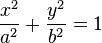
What are elliptic integrals and why are they important? As the name suggests, they are related to ellipses. Given an ellipse of width 2a and height 2b, i.e. satisfying

or using an angular coordinate θ

the arc length along the ellipse from θ = 0 to θ = φ is given by

where m = 1-(a/b)^2 is the so-called elliptic parameter.

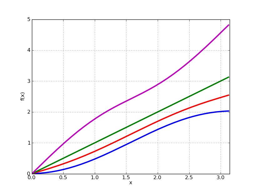
Here are some plots of half-ellipses of various proportions, and the corresponding arc lengths:


a = 1
b1 = 0.1; f1 = lambda x: b1*sqrt(1 - (x/a)**2)
b2 = 0.6; f2 = lambda x: b2*sqrt(1 - (x/a)**2)
b3 = 1.0; f3 = lambda x: b3*sqrt(1 - (x/a)**2)
b4 = 2.0; f4 = lambda x: b4*sqrt(1 - (x/a)**2)
plot([f1,f2,f3,f4], [-1,1])

g1 = lambda phi: b1*ellipe(phi, 1-(a/b1)**2)
g2 = lambda phi: b2*ellipe(phi, 1-(a/b2)**2)
g3 = lambda phi: b3*ellipe(phi, 1-(a/b3)**2)
g4 = lambda phi: b4*ellipe(phi, 1-(a/b4)**2)
plot([g1,g2,g3,g4], [0,pi])

The preceding formulas are sometimes seen with a and b switched, which simply corresponds to transposing x and y as the reference axis (above, the integration is assumed to start on the x axis). One can readily confirm that E(φ, m) satisfies obvious geometric symmetries:


>>> a = 0.5
>>> b = 0.25
>>> m1 = 1-(a/b)**2
>>> m2 = 1-(b/a)**2
>>> b*ellipe(pi/2,m1)           # Arc length of quarter-ellipse
0.6055280137842297624017815
>>> a*ellipe(pi/2,m2)
0.6055280137842297624017815
>>> a*ellipe(pi/4,m2) + b*ellipe(pi/4,m1)
0.6055280137842297624017815
>>> a*ellipe(pi/3,m2) + b*ellipe(pi/6,m1)
0.6055280137842297624017815

Elliptic integrals have countless uses in geometry and physics, and even in pure mathematics. They are related to Jacobi elliptic functions (already available in mpmath), which essentially are inverse functions of elliptic integrals:


>>> m = 0.5
>>> sn = ellipfun('sn')
>>> ellipf(asin(sn('0.65', m)), m)
0.65

More information about elliptic integrals can be found in DLMF Chapter 19.

Implementation

Implementing incomplete elliptic integrals properly is fairly complicated. When people have asked for them in the past, I just suggested using numerical integration. This works quite well most of the time, but it's inefficient (and possibly gives poor accuracy) at high precision, for large arguments, or near singularities. Another approach — computing incomplete integrals from Appell hypergeometric functions (available in mpmath) — basically has the same drawbacks.

The numerically conscious way to compute elliptic integrals is to firstly exploit symmetries to obtain a small standard domain, and then using transformation formulas to reduce the magnitude of the arguments until the first few terms of the hypergeometric series give full accuracy (the arithmetic-geometric mean for the complete integrals, which leads to some of the fastest ways to compute π, is a special case of this process).

The transformations for Legendre's integrals are known as Landen's transformations. A more modern alternative, that I've chosen to use, is to represent Legendre's integrals in terms of Carlson's symmetric integrals which have much simpler structure. Although Carlson's integrals are mainly intended for internal use, I've exposed them as top-level functions since it wasn't much extra work and some users may well find them useful. (Carlson's forms seem to become increasingly standard.)

Carlson's paper is very readable and provides almost complete descriptions of the algorithms, including error bounds, which helped my implementation work tremendously. The error bounds are not rigorous in all cases, but good enough most of the time. Unfortunately, there are many special cases to consider, and Carlson does not address all of them explicitly, so putting it all together nevertheless involved a bit of work (and there are still some minor issues to fix).

Complex branch structure

One major issue is how to define the elliptic integrals for complex (or in some places, negative) parameters. Because the integrands defining Legendre's elliptic integrals involve square roots of periodic functions, they have very complicated branch structure. I have chosen the periodic extension of the branches resulting naturally from use of the Carlson forms on -π/2 < Re(z) < π/2. I believe this is equivalent to choosing the principal-branch square root in the integrand and integrating along a path where the principal branch is continuous.

For example, consider E(φ, 3+4i). The integrand (with the principal square root, as computed by sqrt) and the elliptic integral computed by ellipe are plotted below:

>>> cplot(lambda z: sqrt(1-(3+4j)*sin(z)**2), points=50000)

>>> cplot(lambda z: ellipe(z, 3+4j), points=50000)

It can be seen that the cuts have the same shape in both images (the branch points are necessarily the same). As the following figure shows, if we are to integrate from z = 0 to z = -2+4i (X), a straight path (black) will be bad as it crosses a branch cut (O). However, the modified path (blue) avoiding the branch cut by passing through z = -2 is fine:

We can confirm this with numerical integration:


>>> ellipe(-2+4j, 3+4j)
(36.45544164923053561755261 + 49.28080768743760310823023j)
>>> quad(lambda z: sqrt(1-(3+4j)*sin(z)**2), [0,-2+4j])
(19.65109997738606076596704 + 46.63216059660102110020723j)
>>> quad(lambda z: sqrt(1-(3+4j)*sin(z)**2), [0,-2,-2+4j])
(36.45544164923053561755261 + 49.28080768743760310823023j)

Unfortunately, Mathematica doesn't use quite the same branch cuts for its elliptic integrals. I don't have Mathematica available to create a plot for comparison purposes, but I think it basically uses vertical cuts instead of the curvilinear cuts seen in the images above. There are probably good reasons for doing this, presumably that it simplifies symbolic definite integration, although it seems to complicate the evaluation and formulaic representation of the functions. It would perhaps be good to support both conventions.

As far as the symmetric functions are concerned, they have the nice property that although they involve non-principal square roots (chosen so as to be continuous along the real line), Carlson's algorithm gives the continuous branch automatically. For example, if we consider the first function

with x = i-1, y = i, z = 0, then as the following plot shows, the principal branch of the integrand has a discontinuity at t = 1/2:


>>> x,y,z = j-1,j,0
>>> f = lambda t: 1/sqrt((t+x)*(t+y)*(t+z))
>>> plot(f, [0,3])

To obtain the correct integrand, we switch to the negative square root on the left of the discontinuity (the positive sign should be used on the right because, for continuity with real parameters, we want the principal square root as t → +∞):


>>> g = lambda t: f(t) if t >= 0.5 else -f(t)
>>> plot(g, [0,3])

A quick test shows that f is wrong and g is right:


>>> extradps(25)(quad)(f, [0,inf])/2
(1.110136183412179775397387 - 0.04278194644898641314159222j)
>>> extradps(25)(quad)(g, [0,inf])/2
(0.7961258658423391329305694 - 1.213856669836495986430094j)
>>> elliprf(x,y,z)
(0.7961258658423391329305694 - 1.213856669836495986430094j)

In summary, branch cuts of special functions are a tricky business, and standards don't always exist, so both developers and users need to be careful working with them.

Tuesday, June 15, 2010

Assorted special functions update

Over the week-and-a-half since the last blog update, I've gotten a bunch more work done on special functions in mpmath.

Function plots in the documentation

I have started adding graphics of special functions to the documentation. So far, I've done most of the Bessel-type functions and orthogonal polynomials. Many more to come!

Example screenshot (see the Bessel functions page):

New inhomogeneous Bessel functions

There exists a large number of lesser-known special functions which are essentially variations of Bessel functions. These include functions which solve the generalized (inhomogeneous) Bessel differential equation

with some specific right-hand side g(z). New additions to mpmath in this category are the Anger function (angerj()), Weber function (webere()), and Lommel functions (lommels1(), lommels2()). See commits here and here.

More information about Anger-Weber functions and Lommel functions can be found in the DLMF.

In the near future, I will probably further improve the implementations of the main Bessel functions. The Bessel functions are mostly implemented as generic hypergeometric functions, but the standard cases can be tuned a great deal with special-purpose code.

Airy functions and related functions

The Airy functions Ai and Bi have been present for quite some time in mpmath. In a recent commit, I have rewritten them for improved rigor and better performance at high precision. There are also some new features, such as the ability to evaluate derivatives or iterated integrals of arbitrary order.

Derivatives:


>>> from mpmath import *
>>> mp.dps = 25; mp.pretty = True
>>> airyai(1.5, derivative=5)
0.211387453153454489799743
>>> diff(airyai, 1.5, 5)
0.211387453153454489799743
>>> airyai(1.5, derivative=100)
-6.480220187791312407132043e+49
>>> airybi(0, derivative=1000)
3.754976097101270163249629e+854
>>> airybi(0, derivative=1001)
0.0
>>> airybi(0, derivative=1002)
3.756228172694934424506624e+856

Integrals:


>>> airyai(5, derivative=-1)
0.3332875903059178794866562
>>> quad(airyai, [0,5])
0.3332875903059178794866562
>>> airyai(-100000, derivative=-1)
-0.6665753658794626398413214

Also, functions for computing the zeros of Ai and Bi (and the first derivatives) have been added:


>>> airyaizero(1)
-2.338107410459767038489197
>>> airyaizero(2)
-4.087949444130970616636989
>>> airybizero(1)
-1.17371322270912792491998
>>> airybizero(1, derivative=1)
-2.294439682614123246622459
>>> airybizero(1, derivative=1, complex=True)
(0.2149470745374305676088329 + 1.100600143302797880647194j)
>>> airybizero(10000)
-1304.584974702601410702964
>>> airybizero(10000, complex=True)
(652.3059222438076432024695 + 1129.846189716375208308414j)

I have also implemented two new functions related to Airy functions: the Scorer functions Gi and Hi. These are available as scorergi() and scorerhi() respectively.

Here are two plots of the Gi-function, which can also be seen in the documentation:

Interval gamma functions

The interval arithmetic context now implements gamma, rgamma (reciprocal gamma function), factorial as well as loggamma for real as well as complex arguments (commit). For example:


>>> iv.dps = 10
>>> iv.gamma('50.3')
[1.96282982095908e+63, 1.96282982457481e+63]
>>> iv.gamma(iv.mpc('2.7','5.9'))
([0.00269836072064322, 0.00269836072271801] + 
 [0.0120124287790304, 0.0120124287810768]*j)

As a "practical" example, consider evaluating the Riemann-Siegel theta function which involves computing the difference of two log-gamma functions. For input with a large real part, the imaginary part in the result suffers from massive cancellation and may end up with the wrong sign:


>>> mp.dps = 15
>>> mp.siegeltheta(10**50 + 0.25j)
(5.61456887916465e+51 - 0.143091235731175j)
>>> mp.dps = 10; nprint(mp.siegeltheta(10**50 + 0.25j).imag)
-0.143091
>>> mp.dps = 100; nprint(mp.siegeltheta(10**50 + 0.25j).imag)
14.1614

With interval arithmetic, the sign uncertainty is reflected in the output:


>>> iv.dps = 15
>>> iv.siegeltheta(10**50 + 0.25j)
([5.6145688791646467648e+51, 5.6145688791646474294e+51] +
[-5.0706024009129187319e+30, 5.070602400912917606e+30]*j)
>>> iv.dps = 50
>>> iv.siegeltheta(10**50 + 0.25j)
([5614568879164647368060513633451316140100495086670736.0, 5614568879164647368060
513633451316140100495086670744.0] + 
[14.1613521236438249782320715810808676610440
8814838558203, 14.16147419395632497823207158108086766104408814838560341]*j)

As another example, consider evaluating the gamma function of a huge argument. The digits in the answer may be "wrong" because the input is converted from decimal to binary, and the gamma function is sensitive to the input being perturbed:


>>> mp.dps = 15
>>> mp.gamma('123456789012345.1')
6.11544992055093e+1686076589184486
>>> mp.dps = 30
>>> mp.gamma('123456789012345.1')
7.49032018540342193592769680745e+1686076589184486
>>> mp.dps = 60
>>> mp.gamma('123456789012345.1')
7.49032018540342058679709881225047421518964527875047787194339e+1686076589184486

With interval arithmetic, the uncertainty in the input is propagated correctly:


>>> iv.dps = 15
>>> iv.nprint(iv.gamma('123456789012345.1'), mode='diff')
[6.11545e+1686076589184486, 1.01533e+1686076589184487]
>>> iv.dps = 30
>>> iv.nprint(iv.gamma('123456789012345.1'), 20, mode='diff')
7.4903201854034[185631, 219359]e+1686076589184486
>>> iv.dps = 60
>>> iv.nprint(iv.gamma('123456789012345.1'), 50, mode='diff')
7.49032018540342058679709881225047421518964527[60898, 87505]e+1686076589184486

Rewritten Lambert W function

Lastly, the Lambert W function has received a much-needed rewrite (commit) mainly to improve evaluation very close to the branch cut along the negative axis and particularly near the branch point at -1/e for the k = -1, 0, 1 branches.

With the previous implementation, results were frequently inaccurate or ended up on the wrong branch in this region. Here are some hard cases that now work perfectly:


>>> mp.dps = 1000
>>> x = -1/e + mpf('1e-900')
>>> y = -1/e - mpf('1e-900')
>>> z = -1/e + mpf('1e-900')*1j
>>> w = -1/e - mpf('1e-900')*1j
>>> mp.dps = 25
>>> lambertw(x,0); lambertw(y,0); lambertw(z,0); lambertw(w,0)
-1.0
(-1.0 + 2.331643981597124203363536e-450j)
(-1.0 + 1.648721270700128146848651e-450j)
(-1.0 - 1.648721270700128146848651e-450j)
>>> lambertw(x,1); lambertw(y,1); lambertw(z,1); lambertw(w,1)
(-3.088843015613043855957087 + 7.461489285654254556906117j)
(-3.088843015613043855957087 + 7.461489285654254556906117j)
(-3.088843015613043855957087 + 7.461489285654254556906117j)
(-1.0 + 1.648721270700128146848651e-450j)
>>> lambertw(x,-1); lambertw(y,-1); lambertw(z,-1); lambertw(w,-1)
-1.0
(-1.0 - 2.331643981597124203363536e-450j)
(-1.0 - 1.648721270700128146848651e-450j)
(-3.088843015613043855957087 - 7.461489285654254556906117j)

To finish this post, I present the following Mathematica bug:


remote1:frejohl:[~]$ math
Mathematica 7.0 for Linux x86 (32-bit)
Copyright 1988-2008 Wolfram Research, Inc.

In[1]:= Im[LambertW[0,-1/E-10^(-900)]]

Out[1]= 0

Sunday, June 6, 2010

Announcing mpmath 0.15

I'm happy to announce the release of mpmath 0.15!

This should've happened earlier, but I was obstructed by other obligations (in particular, finishing my master's thesis). The good news is that I will be working full-time on special functions in mpmath and Sage again this summer thanks to sponsorship provided by William Stein (with money from an NSF grant). I will also come to Sage Days 23 (July 5-9, Leiden, the Netherlands) and Sage Days 24 (July 17-22, Linz, Austria) which should be as fun as SD15.

What's new in mpmath 0.15? As usual, the details can be found in the CHANGES file and the list of commits. Most major changes were covered in detail in previous blog posts, so I will first of all simply link to those posts along with short summaries:

Speedups of elementary functions - cos, sin, atan, cosh, sinh, exp and all derived functions are now faster. Of particular note, trigonometric functions use an asymptotically faster algorithm (all elementary functions have similar asymptotic performance now).

A new gamma function implementation - the gamma function and log-gamma functions have been rewritten scratch, using faster algorithms and code optimizations. The new versions are uniformly faster than the old ones, and tens or hundreds of times faster in many important situations. They are also more accurate in some special cases (near singularities, for complex arguments with extremely small real part, ...).

Numerical multidimensional infinite series - nsum() can now evaluate series (finite or infinite) in any number of dimensions

Computing large zeta zeros with mpmath - Juan Arias de Reyna has implemented code for computing the nth zero of the Riemann zeta function on the critical line for arbitrarily large n. On a related note, the Riemann zeta function code has been optimized (mostly through elimination of low-level overhead) to speed up such computations.

Hypergeneralization - generalized 2D hypergeometric series, bilateral hypergeometric series and some q-analogs (q-Pochhammer symbol, q-factorial, q-gamma function, q-hypergeometric series) have been implemented.

In addition, there are many changes that I haven't had time to blog about yet. I will now write briefly about some of these:

Elliptic functions

The support for working with elliptic functions has been improved. Instead of just the standard three, all 12 Jacobi elliptic functions are now available via ellipfun, e.g. the cd-function:


>>> from mpmath import *
>>> mp.dps = 25; mp.pretty = True
>>> ellipfun('cd', 3.5, 0.5)
-0.9891101840595543931308394
>>> cd = ellipfun('cd')
>>> cd(3.5, 0.5)
-0.9891101840595543931308394

Functions qfrom(), qbarfrom(), mfrom(), kfrom(), taufrom() have also been added to convert between the various forms of arguments to elliptic functions (nomes (two definitions), parameters, moduli, half-period ratios). If you're like me and never can remember such formulas, let alone avoid messing up when trying to apply them, this can be quite convenient. Some functions (in particular, ellipfun also support direct choice of convention using keyword arguments):


>>> ellipfun('sn',2,1+1j)    # default is m
(1.333680690847080418060154 - 0.2084318767795699518406447j)
>>> ellipfun('sn',2,q=qfrom(m=1+1j))
(1.333680690847080418060154 - 0.2084318767795699518406447j)
>>> ellipfun('sn',2,k=kfrom(m=1+1j))
(1.333680690847080418060154 - 0.2084318767795699518406447j)
>>> ellipfun('sn',2,tau=taufrom(m=1+1j))
(1.333680690847080418060154 - 0.2084318767795699518406447j)

Another new function is the Klein j-invariant (or rather, the "absolute invariant" or "J-function" which differs by a constant factor, and also is the normalization used by Mathematica). A nice application is to compute the Laurent series expansion in terms of the (number-theoretic) nome, giving a famous integer sequence:


>>> mp.dps = 15
>>> taylor(lambda q: 1728*q*kleinj(qbar=q), 0, 5, singular=True)
[1.0, 744.0, 196884.0, 21493760.0, 864299970.0, 20245856256.0]

The J-function also looks pretty when plotted, here as a function of the number-theoretic nome within the unit circle:


fp.cplot(lambda q: fp.kleinj(qbar=q), [-1,1], [-1,1], points=400000)

As a function of the half-period ratio τ, defined in the upper half-plane:

fp.cplot(lambda t: fp.kleinj(tau=t), [-1,2], [0,1.5], points=100000)

Complex interval arithmetic

The support for interval arithmetic has been extended; there is also a new interface for intervals. It is no longer possible to call mpmath.exp etc. directly with interval arguments; instead all interval arithmetic has been moved to a separate context object called iv (similar to the separate interface for working with Python float/complex in mpmath). For example:


>>> iv.dps = 5; iv.pretty = True
>>> iv.mpf(1)/3
[0.3333330154, 0.3333334923]
>>> iv.sin(1)
[0.8414707184, 0.8414716721]
>>> iv.sin([1,2])
[0.8414707184, 1.0]
>>> iv.sin([1,3])
[0.141119957, 1.0]

The interface change was done to simplify the implementation; separating out interval arithmetic also helps avoid inadvertent mixing of interval and non-interval arithmetic.

There is also some support for complex interval arithmetic, including some elementary functions (exp, log, cos, sin, power).


>>> iv.mpc('1.3','1.4') ** 2
([-0.2700066566, -0.2699956894] + [3.639995575, 3.640010834]*j)
>>> iv.mpc('1.3','1.4') ** iv.mpc('1.2','-0.7')
([3.329280853, 3.329311371] + [1.967472076, 1.967498779]*j)
>>> iv.dps = 25
>>> iv.mpc('1.3','1.4') ** 2
([-0.270000000000000000000000061005, -0.269999999999999999999999912371] +
[3.63999999999999999999999988419, 3.64000000000000000000000009099]*j)
>>> mp.cos(2+3j)
(-4.189625690968807230132555 - 9.109227893755336597979197j)
>>> iv.cos(2+3j)
([-4.18962569096880723013255508975, -4.18962569096880723013255498635] + 
[-9.1092278937553365979791973006, -9.10922789375533659797919709381]*j)

Verifying Euler's identity:


>>> iv.dps = 5
>>> iv.exp(1j * iv.pi)
([-1.0, -0.9999990463] + [-1.279517164e-6, 2.535183739e-6]*j)
>>> iv.dps = 25
>>> iv.exp(1j * iv.pi)
([-1.0, -0.999999999999999999999999987075] +
[-1.8806274411915714063022730148e-26, 3.28925138726485156164403137746e-26]*j)

Rigorous complex linear algebra:


>>> iv.dps = 15
>>> A = iv.matrix([[2,-2,1],[1,0,2],[1,1,2]])
>>> b = iv.matrix([1,2+2j,5])
>>> iv.lu_solve(A,b)
[ ([4.0, 4.0] + [-3.3333333333333333339, -3.333333333333333333]*j)]
[([3.0, 3.0] + [-2.0000000000000000004, -1.9999999999999999998]*j)]
[ ([-1.0, -1.0] + [2.6666666666666666665, 2.666666666666666667]*j)]
>>> A*iv.lu_solve(A,b)
[([1.0, 1.0] + [-8.8817841970012523234e-16, 1.7763568394002504647e-15]*j)]
[         ([2.0, 2.0] + [1.9999999999999995559, 2.0000000000000008882]*j)]
[([5.0, 5.0] + [-8.8817841970012523234e-16, 1.7763568394002504647e-15]*j)]

Partial derivatives

This is rather simple, but very convenient. diff can now compute partial derivatives of arbitrary order for multivariable functions. For example, a first derivative with respect to the second argument:


>>> diff(lambda x,y: 3*x*y + 2*y - x, (0.25, 0.5), (0,1))
2.75

The first derivative with respect to both x and y:


>>> diff(lambda x,y: 3*x*y + 2*y - x, (0.25, 0.5), (1,1))
3.0

Second derivative with respect to a parameter of a hypergeometric function ₂F₁(a,b,c,z); tenth derivative with respect to the argument; first derivative with respect to two parameters and fourth derivative with respect to the argument:


>>> diff(hyp2f1, (1,2,3,0.5), (0,0,2,0))
0.2306514802159766624657329
>>> diff(hyp2f1, (1,2,3,0.5), (0,0,0,10))
672869392.1810426015397572
>>> diff(hyp2f1, (1,2,3,0.5), (1,0,1,4))
-585.1335939248098118753126

That's it for now. Stay tuned for many new features in the near future!

Wednesday, March 17, 2010

Hypergeneralization

The generalized hypergeometric function can itself be generalized endlessly. I have recently implemented three such extensions in mpmath: bilateral series, two-dimensional hypergeometric series, and q-analog (or "basic") hypergeometric series.

Bilateral series

The bilateral hypergeometric series is the simplest extension, and consists of taking the usual hypergeometric series and extending the range of summation from [0,∞) to (-∞,∞):

This series only converges when |z| = 1 and A = B, but interpreted as a sum of two ordinary hypergeometric series, it can be assigned a value for arbitrary z through the analytic continuation (or Borel regularization) of the ordinary hypergeometric series, which mpmath implements. Anyway, the convergent case is the interesting one. Here one obtains, for instance, Dougall's identity for 2H2:


>>> from mpmath import *
>>> mp.dps = 25; mp.pretty = True
>>> a,b,c,d = 0.5, 1.5, 2.25, 3.25
>>> bihyper([a,b],[c,d],1)
-14.49118026212345786148847
>>> gammaprod([c,d,1-a,1-b,c+d-a-b-1],[c-a,d-a,c-b,d-b])
-14.49118026212345786148847

As an example of regularization, the divergent 1H0 series can be expressed as the sum of one 2F0 function and one 1F1 function:


>>> a = mpf(0.25)
>>> z = mpf(0.75)
>>> bihyper([a], [], z)
(0.2454393389657273841385582 + 0.2454393389657273841385582j)
>>> hyper([a,1],[],z) + (hyper([1],[1-a],-1/z)-1)
(0.2454393389657273841385582 + 0.2454393389657273841385582j)
>>> hyper([a,1],[],z) + hyper([1],[2-a],-1/z)/z/(a-1)
(0.2454393389657273841385582 + 0.2454393389657273841385582j)

Two-dimensional series

The most common hypergeometric series of two variables, i.e. a twodimensional series whose summand is a hypergeometric expression with respect to both indices separately, is the Appell F1 function, previously available in mpmath as appellf1:

However, much more general functions are possible. There are three other Appell functions: F2, F3, F4. The Horn functions are 34 distinct functions of order two, containing the Appell functions as special cases. The Kampé de Fériet function provides a generalization of Appell functions to arbitrary orders.

The new hyper2d function in mpmath can evaluate all these named functions, and more general functions still. The trick for speed is to write the series as a nested series, where the inner series is a generalized hypergeometric series that can be evaluated efficiently with hyper, and where the outer series has a rational recurrence formula. This rewriting also permits evaluating the analytic continuation with respect to the inner variable (as implemented by hyper).

The user specifies the format of the series in quasi-symbolic form, and the rewriting to nested form is done automatically by mpmath. For example, the Appell F1 function can be computed as


hyper2d({'m+n':[a], 'm':[b1], 'n':[b2]}, {'m+n':[c]}, x, y)

and indeed, this is essentially what appellf1 now does internally. The Appell F2-F4 functions have also been added explicitly as appellf2, appellf3, appellf4.

Hypergeometric functions of two (or more) variables have numerous applications, such as solving high-order algebraic equations, expressing various derivatives and integrals in closed form, and solving differential equations, but I have not yet found any simple examples that make good demonstrations except for F1. (I have mostly found examples of that take half a page to write down.) Any such examples for the documentation would be a welcome contribution!

Some trivial examples from the documentation are:


>>> x, y = mpf(0.25), mpf(0.5)
>>> hyper2d({'m':1,'n':1}, {}, x,y)
2.666666666666666666666667
>>> 1/(1-x)/(1-y)
2.666666666666666666666667
>>> hyper2d({'m':[1,2],'n':[3,4]}, {'m':[5],'n':[6]}, x,y)
4.164358531238938319669856
>>> hyp2f1(1,2,5,x)*hyp2f1(3,4,6,y)
4.164358531238938319669856
>>> hyper2d({'m':1,'n':1},{'m+n':1},x,y)
2.013417124712514809623881
>>> (exp(x)*x-exp(y)*y)/(x-y)
2.013417124712514809623881

An example of a Horn function, H3:


>>> x, y = 0.0625, 0.125
>>> a,b,c = 0.5,0.75,0.625
>>> hyper2d({'2m+n':a,'n':b},{'m+n':c},x,y)
1.190003093972956004227425
>>> nsum(lambda m,n: rf(a,2*m+n)*rf(b,n)/rf(c,m+n)*\
...     x**m*y**n/fac(m)/fac(n), [0,inf], [0,inf])
1.190003093972956004227425

This also demonstrates the recently added generic support for multidimensional infinite series in mpmath. But of course, nsum is much slower than hyper2d.

Hypergeometric q-series

Before introducing the q-analog of the hypergeometric series, I should introduce the q-Pochhammer symbol,

This itself is a new function in mpmath, implemented as qp(a,q,n) (with two- and one-argument forms qp(a,q) and qp(q) also permitted) and is the basis for more general computation involving q-analogs. The q-factorial and q-gamma function have also been added (as qfac and qgamma), but are not yet documented.

The q-analogs have important applications in number theory. As a very neat example, numerically computing the Taylor series of 1/(q, q)_∞ with mpmath gives


>>> taylor(lambda q: 1/qp(q), 0, 10)
[1.0, 1.0, 2.0, 3.0, 5.0, 7.0, 11.0, 15.0, 22.0, 30.0, 42.0]

These are the values of the partition function P(n) for n = 0,1,2,..., i.e. the number of ways of writing n as a sum of positive integers.

Replacing the rising factorials (Pochhammer symbols) in the generalized hypergeometric series with their q-analogs gives the hypergeometric q-series or basic hypergeometric series

This function is implemented as qhyper. Like hyper, it supports arbitrary combinations of real and complex arguments (assuming |q| < 1). Some examples from the documentation:


>>> qhyper([0.5], [2.25], 0.25, 4)
-0.1975849091263356009534385
>>> qhyper([0.5], [2.25], 0.25-0.25j, 4)
(2.806330244925716649839237 + 3.568997623337943121769938j)
>>> qhyper([1+j], [2,3+0.5j], 0.25, 3+4j)
(9.112885171773400017270226 - 1.272756997166375050700388j)

Like hyper, it automatically ensures accurate evaluation for alternating series:


>>> q = 0.998046875
>>> mp.dps=5; qhyper([2],[0.5], q, -0.5)
6.6738e-69
>>> mp.dps=15; qhyper([2],[0.5], q, -0.5)
6.67376764851253e-69
>>> mp.dps=25; qhyper([2],[0.5], q, -0.5)
6.673767648512527695718826e-69
>>> mp.dps=100; qhyper([2],[0.5], q, -0.5)
6.673767648512527695718826106778799352769798151218768443717704076836963752188876
561888441662933081804e-69

With the q-analog of the generalized hypergeometric function implemented, it becomes possible to compute q-exponentials, q-sines, q-orthogonal polynomials, q-Bessel functions, and pretty much anything else. If there is interest, such function could be added explicitly to mpmath.

For more information and examples of the functions discussed in this post, see the sections on hypergeometric functions and q-functions (a little terse at the moment) in the mpmath documentation.

Friday, March 12, 2010

Computing large zeta zeros with mpmath

Juan Arias de Reyna, who wrote the code used in mpmath for evaluating the Riemann zeta function near the critical strip, has contributed a new implementation of the zetazero function which computes the nth zero on the critical line.

The old version (written by myself) used a lookup table for initial approximations, so it was limited to computing the first few zeros. Juan's code calculates the position of arbitrary zeros using Gram's law, with a sophisticated algorithm (about 300 lines of code) to find the correct zero when Gram's law (which is actually just a heuristic) fails.

A bunch of zeros, from small to large:


from mpmath import *
from timeit import default_timer as clock
mp.dps = 20
for n in range(14):
    t1 = clock()
    v1 = zetazero(10**n)
    t2 = clock()
    v2 = zetazero(10**n+1)
    t3 = clock()
    print "10<sup>%i</sup>  "%n, v1, "%.2f" % (t2-t1)
    print "10<sup>%i</sup>+1"%n, v2, "%.2f" % (t3-t2)


n      value                          time (s)
10⁰    (0.5 + 14.13472514173469379j)  0.12
10⁰+1  (0.5 + 21.022039638771554993j) 0.05
10¹    (0.5 + 49.773832477672302182j) 0.05
10¹+1  (0.5 + 52.970321477714460644j) 0.04
10²    (0.5 + 236.5242296658162058j)  0.32
10²+1  (0.5 + 237.769820480925204j)   0.30
10³    (0.5 + 1419.4224809459956865j) 0.93
10³+1  (0.5 + 1420.416526323751136j)  0.84
10⁴    (0.5 + 9877.7826540055011428j) 3.75
10⁴+1  (0.5 + 9878.6547723856922882j) 3.71
10⁵    (0.5 + 74920.827498994186794j) 2.53
10⁵+1  (0.5 + 74921.929793958414308j) 2.58
10⁶    (0.5 + 600269.67701244495552j) 2.43
10⁶+1  (0.5 + 600270.30109071169866j) 2.89
10⁷    (0.5 + 4992381.014003178666j)  1.63
10⁷+1  (0.5 + 4992381.2627112065366j) 2.30
10⁸    (0.5 + 42653549.760951553903j) 2.36
10⁸+1  (0.5 + 42653550.046758478876j) 2.93
10⁹    (0.5 + 371870203.83702805273j) 6.98
10⁹+1  (0.5 + 371870204.36631304458j) 6.72
10¹⁰   (0.5 + 3293531632.3971367042j) 11.48
10¹⁰+1 (0.5 + 3293531632.6869557853j) 15.92
10¹¹   (0.5 + 29538618431.613072811j) 53.67
10¹¹+1 (0.5 + 29538618432.07777426j)  43.00
10¹²   (0.5 + 267653395648.62594824j) 162.01
10¹²+1 (0.5 + 267653395648.84752313j) 174.67
10¹³   (0.5 + 2445999556030.2468814j) 1262.55
10¹³+1 (0.5 + 2445999556030.6222451j) 1456.38

The function correctly separates close zeros, and can optionally return information about the separation. For example:


>>> mp.dps = 20; mp.pretty = True
>>> zetazero(542964976,info=True)
((0.5 + 209039046.578535272j), [542964969, 542964978], 6, '(013111110)')

The extra information is explained in the docstring for zetazero:

[This means that the] zero is between Gram points 542964969 and 542964978, it is the 6-th zero between them. Finally (01311110) is the pattern of zeros in this interval. The numbers indicate the number of zeros in each Gram interval, (Rosser Blocks between parenthesis). In this case only one Rosser Block of length nine.

Juan reports having computed the 10¹⁵th zero, which is


208514052006405.46942460229754774510611

and verifying that it satisfies the Riemann hypothesis. And fortunately, the values of large zeros computed with mpmath seem to agree with those reported by Andrew Odlyzko and Xavier Gourdon.

The new zetazero function in mpmath is indeed able to separate the closest known pair of zeros, found in Xavier Gourdon's exhaustive search up to 10¹³:


>>> mp.dps = 25
>>> v1 = zetazero(8637740722917, info=True)
>>> v2 = zetazero(8637740722918, info=True)
>>> v1
((0.5 + 2124447368584.392964661515j), [8637740722909L, 8637740722925L], 7L,
'(1)(1)(1)(1)(1)(1)(02)(1)(02)(1)(1)(20)(1)')
>>> v2
((0.5 + 2124447368584.392981706039j), [8637740722909L, 8637740722925L], 8L,
'(1)(1)(1)(1)(1)(1)(02)(1)(02)(1)(1)(20)(1)')
>>> nprint(abs(v1[0]-v2[0]))
1.70445e-5

This computation takes over 2 hours on my laptop.

Of course, zeros can be computed to any desired precision:


>>> mp.dps = 1000
>>> print zetazero(1)
(0.5 + 14.1347251417346937904572519835624702707842571156992431756855674601499634
29809256764949010393171561012779202971548797436766142691469882254582505363239447
13778041338123720597054962195586586020055556672583601077370020541098266150754278
05174425913062544819786510723049387256297383215774203952157256748093321400349904
68034346267314420920377385487141378317356396995365428113079680531491688529067820
82298049264338666734623320078758761792005604868054356801444424651065597568665903
22868651054485944432062407272703209427452221304874872092412385141835146054279015
24478338354254533440044879368067616973008190007313938549837362150130451672696838
92003917628512321285422052396913342583227533516406016976352756375896953767492033
61272092599917304270756830879511844534891800863008264831251691127106829105237596
17977431815170713545316775495153828937849036474709727019948485532209253574357909
22612524773659551801697523346121397731600535412592674745572587780147260983080897
860071253208750939599796666067537838121489190886j)

The only real limitation of the code, as far as I can tell, is that it's impractical for computing a large number of consecutive zeros. For that one needs to use something like the Odlyzko–Schönhage algorithm for multi-evaluation of the zeta function.

A nice exercise would be to parallelize the zeta code using multiprocessing. The speedup for large zeros should be essentially linear with the number of processors.

Thursday, March 11, 2010

Speedups of elementary functions

I have a fairly large backlog of changes in mpmath to blog about. For today, I'll just briefly mention the most recent one, which is a set of optimizations to elementary functions. The commit is here. I intend to provide much faster Cython versions of the elementary functions some time in the future, but since there was room for optimizing the Python versions, I decided to invest a little time in that.

Most importantly, the asymptotic performance of trigonometric function has been improved greatly, due to a more optimized complexity reduction strategy. The faster strategy was previously used only for exp, but cos/sin are virtually identical in theory so fixing this was mostly a coding problem. In fact, the high-precision code for exp/cosh/sinh/cos/sin is largely shared now, which is nice because only one implementation needs to be optimized.

The following image shows performance for computing cos(3.7). The red graph is the old implementation; blue is new. The top subplot shows evaluations/second at low precision, i.e. higher is better, and the bottom subplot shows seconds/evaluation at higher precision, i.e. lower is better.

Already at a few thousand bits, the new code is more than twice as fast, and then it just gets better and better. There is also a little less overhead at low precision now, so the new code is uniformly faster.

Also exp, cosh and sinh have been optimized slightly. Most importantly, there is a little less overhead at low precision, but asymptotic speed has also improved a bit.

Performance for computing cosh(3.7):

Performance for computing exp(3.7):

I should note that the performance depends on some tuning parameters which naturally are system-specific. The results above are on a 32-bit system with gmpy as the backend. I hope to later implement optimized tuning parameters for other systems as well.

Elementary function performance is of course important globally, but it's especially important for some specific functions. For example, the speed of the Riemann zeta function depends almost proportionally on the total speed of evaluating one exp, one log, one sine, and one cosine, since the main part of the work consists of summing the truncated L-series

With the improved elementary functions, and some overhead removals to the zetasum code in the same commit, the Riemann zeta function is up to 2x faster now, and about 50% faster on the critical line.